In probability theory, one is often interested in the question of whether or not a joint distribution arises from two independent variables or whether or not the variables are correlated. In this post, we consider (an aspect) of the geometry of this question in the case of 4D joint distributions

Geometrically, an \(n\)-dimensional probability distributions live on the \(n\)-dimensional simplex, \(\Delta_n\) defined to be the set $$ \Delta_n = \Big\{ x \in \mathbb{R}^n \ \ \big| \ \ \mathbf{1}^\top x = 1, \ \ x \geq 0 \Big\} $$ where \(\mathbf{1}\) is a vector of all ones of dimension \(n\) and the inequality is taken elementwise. The probability simplicies in 2D,3D, and 4D are shown here.

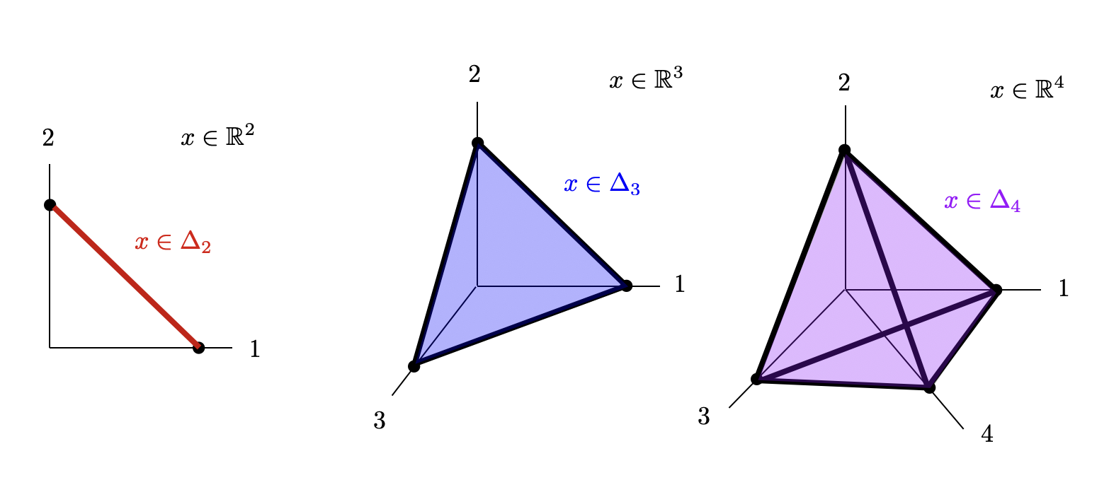
Note that the simplex itself in each space has dimension one lower than the ambient space (due to the affine constraint \(\mathbf{1}^\top x = 1\). For example, the simplex in 2D is a 1D line segment, the simplex in 3D is a 2D triangle, and the simplex in 4D is a 3D tetrahedron. Each set has corners at the standard basis vectors and is bounded away from the origin. Higher dimensional probability distributions often arise as product or joint-distributions from lower dimensional independent distributions. For example, consider two independent scenarios each with \(n\) outcomes with probabilities given by the elements of \(x \in \Delta_n\) for Scenario 1 and \(y \in \Delta_n\) for Scenario 2. If the two scenarios are independent, the probability of event \(i\) happening for Scenario 1 and event \(j\) happening for Scenario 2 is given by \(Z_{ij} = x_i y_j\). We can specify the joint distribution of every possible combination of events as an \(n\times n\) matrix $$ Z = xy^\top \in \mathbb{R}^{n \times n} $$ Note that \(Z\) is a valid probability distribution since \(Z_{ij} \geq 0\) for all \(i,j\) and $$ \sum_{ij} Z_{ij} = \mathbf{1}^\top Z \mathbf{1} = (\mathbf{1}^\top x) (y^\top \mathbf{1}) = 1 \cdot 1 = 1 $$ Since \(Z\) is a matrix, to be consistent we will talk about it's vectorized form, \(\text{vec}(Z)\) as living on the simplex in \(\mathbb{R}^{n^2}\) $$ \text{vec}(Z) \in \Delta_{n^2} = \Big\{ \ \ \text{vec}(Z) \ \ \big| \ \ \mathbf{1}^\top \text{vec}(Z) = 1, \ \ \text{vec}(Z) \geq 0 \Big\} $$ We can now make some comments about the full set of joint distributions (both independent and dependent) vs. the subset of independent distributions. The full probability simplex in dimension \(n^2\) is a polytope of dimension \(n^2 - 1\) since, again, it is defined by a single affine constraint. The set of independent distributions is associated with the rank-1 matrices defined above and is determined by the degrees of freedom in \(x\) and \(y\), ie. \(2n\) degrees-of-freedom. In the remainder of this post, we will examine the geometry of these sets in a low dimensional setting and specifically, we will see that the set of independent is a particular non-convex surface in the full joint-distribution simplex.

We now consider the case where \(x,y \in \Delta_2 \). We consider the set of independent joint-distributions of the form \(Z = xy^\top \). Vectorized, this set can be defined as a subset of \(\Delta_4\) as follows $$ \mathcal{I} = \Big\{\ \ \text{vec}(Z) \in \mathbb{R}^4 \ \ \big| \ \ Z = xy^\top, \ x \in \Delta_2, \ y \in \Delta_2 \Big\} \subset \Delta_4 $$ For the sake visualization, note that we can parametrize \(\Delta_2\) in the following way $$ \Delta_2 = \Bigg\{ \ \ x \in \mathbb{R}^2 \ \ \bigg| \ \ x = \begin{bmatrix} 1 \\ 0 \end{bmatrix} u + \begin{bmatrix} 0 \\ 1 \end{bmatrix}(1-u), \ 0 \leq u \leq 1, \ u \in \mathbb{R} \Bigg\} $$ Using this parametrization on both \(x \in \Delta_2\) and \(y \in \Delta_2\) with two separate scalar parameters \(u\) and \(v\) both in \([0,1]\), we can parametrize the set \(\mathcal{I}\) as well $$ \begin{aligned} \mathcal{I} = \Bigg\{\ \ \text{vec}(Z) \in \mathbb{R}^4 \ \ \bigg| \ \ Z = & \underbrace{ \begin{bmatrix} 1 & 0 \\ 0 & 0 \end{bmatrix}}_{a} uv+ \underbrace{ \begin{bmatrix} 0 & 1 \\ 0 & 0 \end{bmatrix}}_{b} u(1-v) \\ & + \underbrace{\begin{bmatrix} 0 & 0 \\ 1 & 0 \end{bmatrix}}_{c} (1-u)v + \underbrace{ \begin{bmatrix} 0 & 0 \\ 0 & 1 \end{bmatrix}}_{d} (1-u)(1-v), \ u,v \in [0,1] \Bigg\} \end{aligned} $$ Although, we can't easily plot the 4D vectors labeled \(a,b,c,d\) above we can simply plot a similar parametrization with \(a,b,c,d\) each assigned to a 3D vector. (Since \(\Delta_4\) is actually a 3D polytope no information is lost in doing this.) For no particular reason, we define the four corners of the tetrahedron as the points \(a,b,c,d \in \mathbb{R}^3\) $$ a = \begin{bmatrix}1 \\ -0.3 \\ 0 \end{bmatrix}, \quad b = \begin{bmatrix}-0.3 \\ 1 \\ 0 \end{bmatrix}, \quad c = \begin{bmatrix} 0 \\ 0 \\ 1.3 \end{bmatrix}, \quad d = \begin{bmatrix}-0.7 \\ -0.7 \\ 0. \end{bmatrix} $$ We show this visualization here.

https://www.desmos.com/3d/a106c8ceb2

In the visualization, we also plot out the edges of the tetrahedron for clarity.

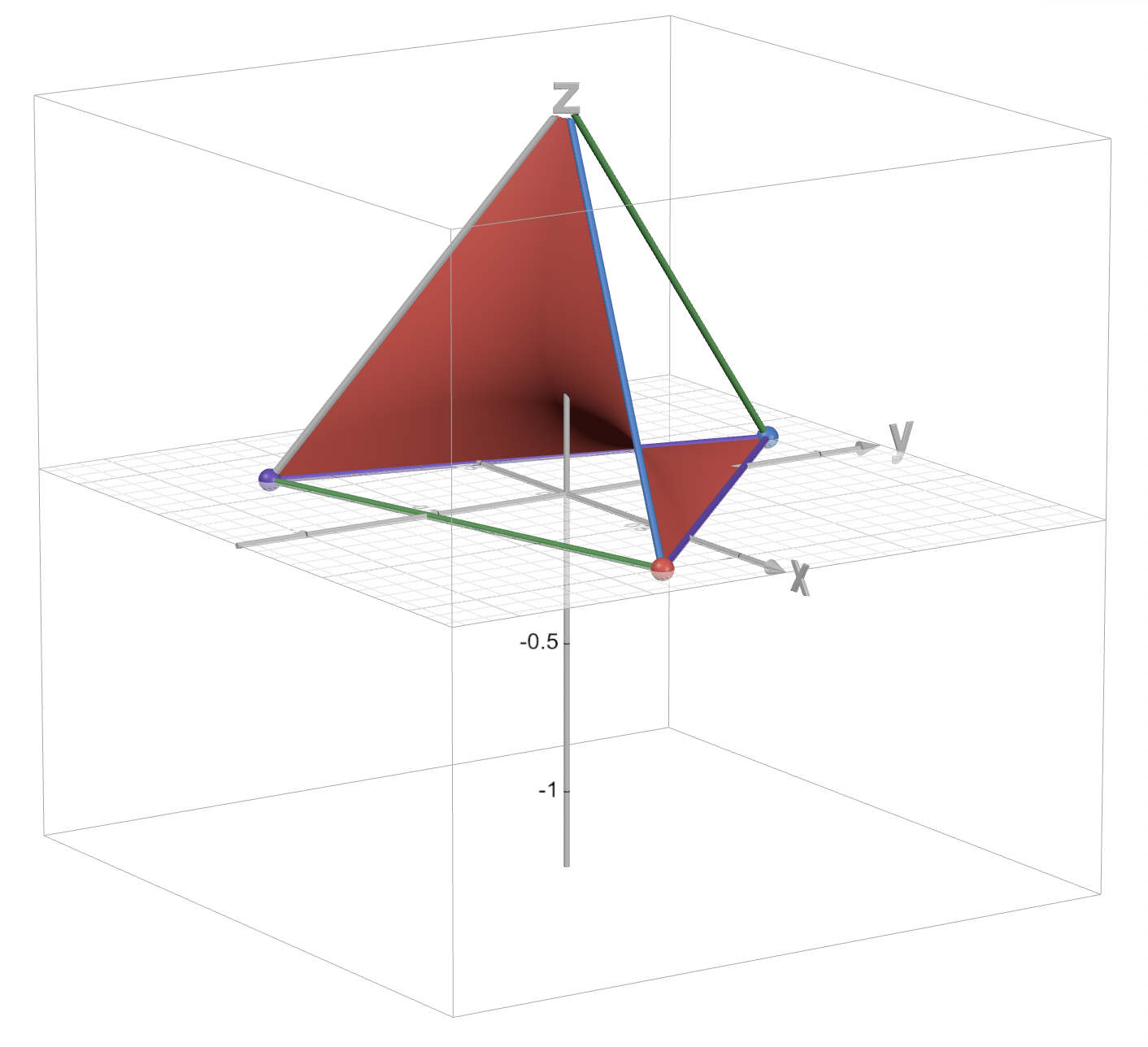
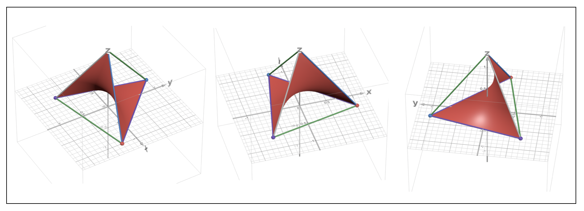
A couple things to note: as expected the red surface \(\mathcal{I}\) is contained inside the simplex. It is also clearly a nonlinear surface as a result of the multi-linear structure \(L=xy^\top\).