Problem Setup

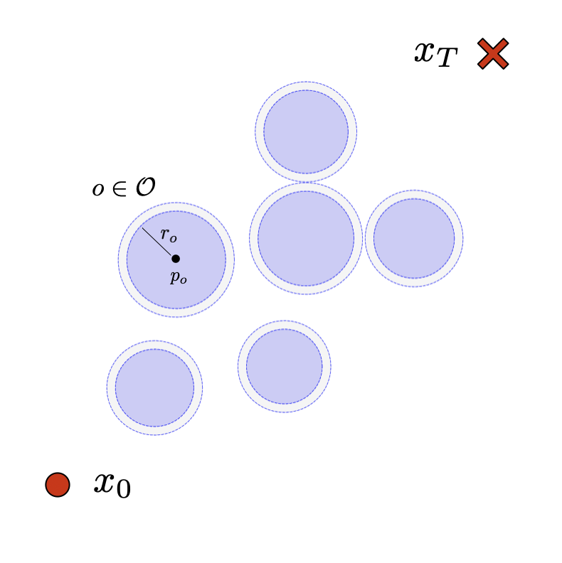
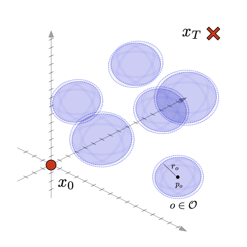
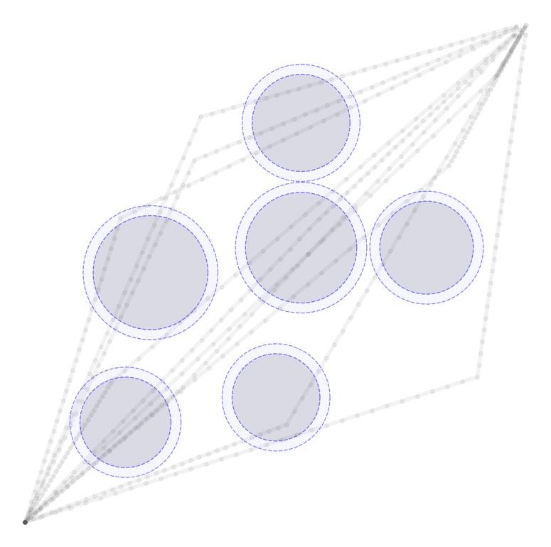
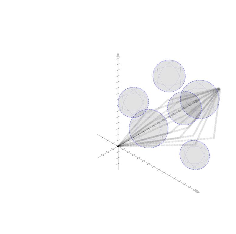
We consider a basic trajectory planning problem to get between two points. We want to find a path between the starting and end point consistent with the dynamcis while avoiding a set of obstacles denotes \(\mathcal{O}\). We will consider state vector \(x(t) \in \mathbb{R}^n\) for \(n=2,3\) and controls \(u(t) \in \mathbb{R}^n\) for \(n=2,3\) as well. We will consider simple spherical obstacles with centers \(p_o \in \mathbb{R}^{n}\) and radii \(r_o \in \mathbb{R}_+\). The starting and ending locations at times 0 and T respectively will be given. We display two such simple environments in 2D and 3D here.

Dynamics:

In order to focus on the most basic trajectory planning, we start with the most basic, single-integrator dynamics $$ \begin{aligned} \dot{x}(t) = f(x,u,t) = u(t) \end{aligned} $$ We can now compute the discrete time dynamics $$ \begin{aligned} x(t+\Delta t) & = Ax(t) + Bu(t) \\ & = x(t) + \int_0^{\Delta t} B u(\tau) \ d\tau = I + \Delta t \ u(t) \end{aligned} $$ where here \(A \in \mathbb{R}^{n \times n} \) and \(B \in \mathbb{R}^{n \times n}\) are the discrete time LTI matrices with \(A = e^{0\Delta t} = I\) and \(B=\Delta t I \). In this simple case, the Forward-Euler integration scheme (on the right) is precise assuming a first-order hold of the control input over the time step. We can also compute the reachability matrix for \(k\) time steps. $$ \begin{aligned} M_k & = \Big[ A^{k-1}B \ A^{k-2}B \ \cdots \ AB \ B \Big] \\ & = \Delta t \Big[ \ I \ \ I \ \ \cdots \ \ I \ \ I \ \Big] \end{aligned} $$ We will use \(\mathbf{x} \in \mathbb{R}^{nT}\) and \(\mathbf{u} \in \mathbb{R}^{nT}\)to represent the rolled out state and control trajectories $$ \begin{aligned} \mathbf{x} & = \Big(x\big(0\big),x\big(\Delta t\big),\dots,x\big(\Delta t T\big)\Big), \quad \mathbf{u} = \Big(u\big(0\big),u\big(\Delta t\big),\dots,u\big(\Delta t (T-1)\big)\Big) \end{aligned} $$ We can integrate out a control trajectory get the dynamics as $$ \begin{aligned} x(k\Delta t ) & = x_0 + \sum_{j=0}^{k-1} A^{k-1-j} B u(j\Delta t) + x_0 \\ & = x_0 + \sum_{j=0}^{k-1} \Delta t u(j\Delta t) \end{aligned} $$ In vector form this can be written as $$ \begin{aligned} \mathbf{x} = \mathbf{H} x_0 + \mathbf{M} \mathbf{u} \end{aligned} $$ where \(\mathbf{H} \in \mathbb{R}^{nT \times n}\) and \(\mathbf{M} \in \mathbb{R}^{nT\times nT}\) are given by $$ \begin{aligned} \mathbf{H} = \begin{bmatrix} I \\ I \\ I \\ I \\ \vdots \\ I \end{bmatrix}, \quad \mathbf{M} = \begin{bmatrix} 0 & 0 & 0 & \cdots & 0 \\ B & 0 & 0 & \cdots & 0 \\ AB & B & 0 & \cdots & 0 \\ A^2B & AB & B & \cdots & 0 \\ \vdots & \vdots & \vdots & \ddots & \vdots \\ A^{T-1}B & A^{T-2}B & A{T-3}B & \cdots & B \end{bmatrix} \end{aligned} $$

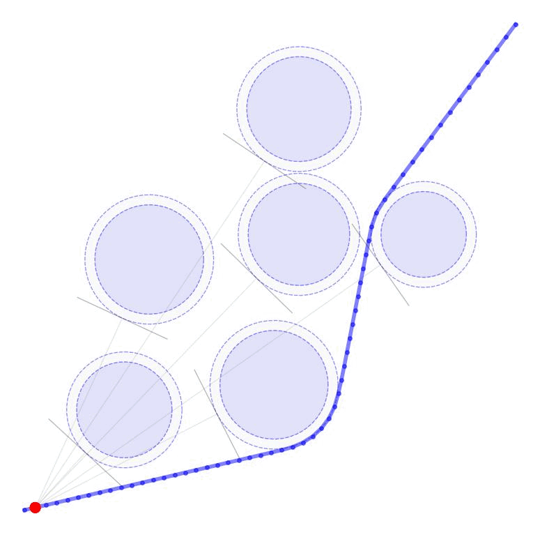
Initial Control and Trajectory

We first come up with an initial control trajectory, \(\mathbf{u}^{(0)}\), that drives us from the origin to the destination by finding a minimum norm control scheme. We want to satisfy the equation $$ \begin{aligned} x_T = x_0 + M_T\mathbf{u}^{(0)} \end{aligned} $$ Since \(M_T\) is a fat matrix this equation has a subspace of solutions; we can find the minimum norm solution by computing $$ \begin{aligned} \mathbf{u}^{(0)} = M_T^\top(M_TM_T^\top)^{-1}(x_T - x_0) \end{aligned} $$ In order to compute a diversity of possible trajectories, we may make an additional modification and force trajectories to pass through an intermediate state at the mid point of the time horizon. If we define this intermediate state as \(x_{T/2}\) and consider a reachability matrix for just half of the time horizon, \(M_{T/2}\), we can define the initial minimum norm control (passing through the intermediate point) as $$ \begin{aligned} \mathbf{u}^{(0)} = \begin{bmatrix} M_{T/2}^\top(M_{T/2}M_{T/2}^\top)^{-1}(x_{T/2} - x_0), \\ M_{T/2}^\top(M_{T/2}M_{T/2}^\top)^{-1}(x_T - x_{T/2}) \end{bmatrix} \end{aligned} $$ The initial state trajectories \(\mathbf{x}^(0)\) can then be computed by integrating the initial contols. Several such trajectories are shown here passing through their random middle points.

Note that in computing the initial control and state trajectories we have ignored the obstacles and we will need to fix this in the next step.

CONVEX SUBPROBLEM

We now want seek to improve our trajectories so that 1) the obstacles are avoided and 2) we reduce the amount of control effort that is employed. We use the successive convexification scheme developed by Behcet Ackimese and company. At each update iteration we will solve the following optimization problem for a given, nominal control and state trajectories \(\mathbf{x}\) and \(\mathbf{u}\). $$ \begin{aligned} \textbf{OPT}\big(\mathbf{u},\mathbf{x}\big) = \min_{\partial u,\partial x} & \quad w_u \sum_k (u_k+\partial u_k)^\top R_k (u_k+\partial u_k) + w_s\sum_k v_k^\top v_k \\ \text{s.t.} & \quad \partial x_{k+1} = A_k \partial x_k + B_k \partial u_k, \ \quad \forall k \\ & \quad \partial x_0 = 0, \ \partial x_T = 0 \\ & \quad G_k \partial x_k \leq d_k + v_k \geq 0, \ v_k \geq 0 \quad \forall k \end{aligned} $$ We now break down each element of the optimization problem.

Linearized Dynamics

Perturbations of the state trajectory around the nominal trajectory will obey a linearized version of the dynamics. At each time step, the matrices \(A_k\) and \(B_k\) are the Jacobians of the dynamcis with respect to the state and the control $$ A_k = I + \Delta t \frac{\partial f}{\partial x_k}, \qquad B_k = \Delta t \frac{\partial f}{\partial u_k} $$ We also force the perturbations of the initial and final state to be zero, ie. \(\partial x_0 = 0\) and \(\partial x_T = 0 \), so that the desired initial and final states are maintained.

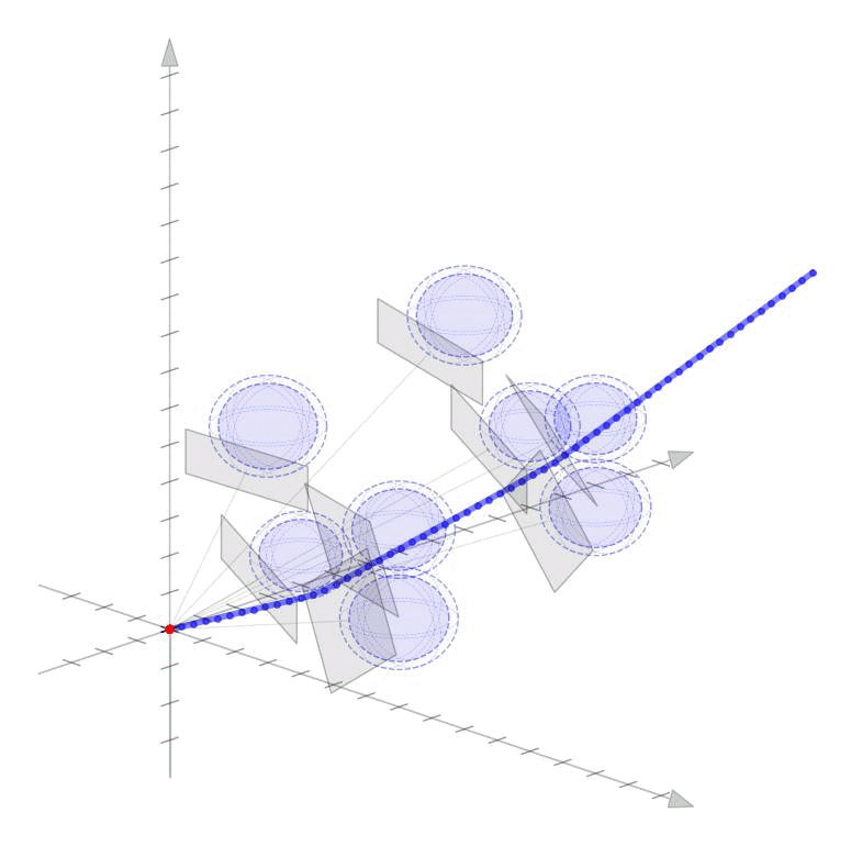
Linearized Boundary Constraints

At each time step, we consider a linearized version of the constraint posed by each of the obstacles for the state at that time step. Specifically, we can force the state perturbation at time step \(k\), \(\partial x_k\), to satisfy the linear constraint $$ \begin{aligned} G_k \partial x_k \leq d_k + v_k 0, \quad v_k \geq 0 \end{aligned} $$ Here \(G \in \mathbb{R}^{|\mathcal{O}|\times n}\) is matrix whose rows give the normal directions toward the surface of each obstacle given the current estimate of \(x_k\) and the elements of \(d_k \in \mathbb{R}^{|\mathcal{O}|}\) gives the distance to each obstacle $$ \begin{aligned} G_k = \begin{bmatrix} - & G_{1k} & - \\ & \vdots & \\ - & G_{|\mathcal{O}|k} & - \\ \end{bmatrix}, \qquad d_k = \begin{bmatrix} d_{1k} \\ \vdots \\ d_{|\mathcal{O}|k} \end{bmatrix}, \end{aligned} $$ as displayed in these figures in 2D and 3D.

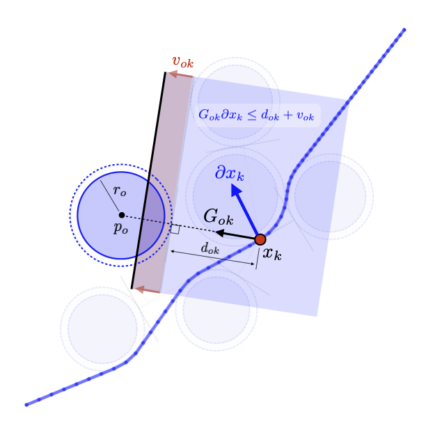
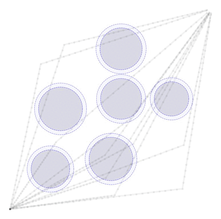
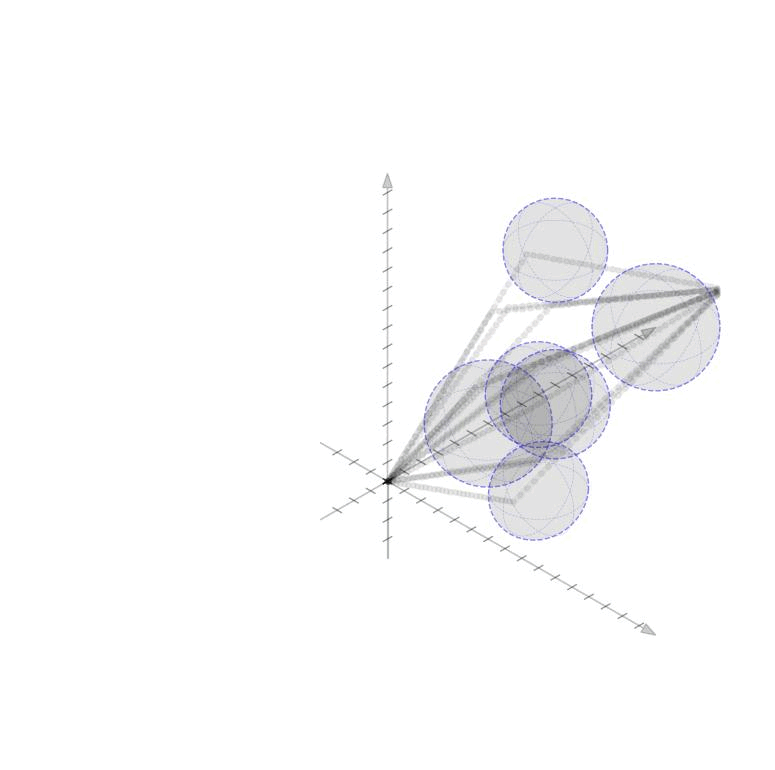
Each row of \(G_k\) and each element of \(d_k\) can be computed as $$ \begin{aligned} G_{ok} = \frac{p_o - x_k}{||p_o - x_k||}, \qquad d_{ok} = ||p_o - x_k|| - r_o \end{aligned} $$ where \(p_o \in \mathbb{R}^n\) is the position of each obstacle and \(r_o \in \mathbb{R}_+\) is the radius of each obstacle. The additional variable \(v_{ok}\) (vectorized as \(v_k \in \mathbb{R}^{|\mathcal{O}|}\)) is a buffer variable that allows the constraints to be violated at intermediate iterations; we will, however, penalize these buffer variables heavily in the objective function to push the trajectory outside the obstacles. To be conservative, we can also provide a buffer around the obstacles as well to keep our trajectory away from them. In the following figures, we illustrate the linearized constraints at each time step along the state trajectory. Note that the perturbed state at each time step is bounded by a different set of hyperplanes that approximate the location of the obstacle relative to the current estimate of that particular state.

Objective Function

The simplest version of the objective function penalizes two things. 1) We penalize the buffer variables on the constraints to push the trajectory outside the obstacles. 2) We penalize the total control input \(u_k + \partial u_k\) to minimize the total control effort. The weighting variables \(w_u\) and \(w_v\) provide the relative penalty on the control effort and satisfying the constraints. In general, we will want \(w_v\) to be substantially higher than \(w_u\) to ensure that the constraints are satisfied. In these examples, we set \(w_u = 1\) and \(w_v = 1000\).

SUCCESSIVE CONVEXIFICATION

The algorithm will then proceed as follows. First, we initialize \(i=0\) and \(\mathbf{u}^{(0)}\) as described above. We then perform the following iterations $$ \begin{aligned} \text{Integrate: } & \quad \mathbf{u}^{(i)} \Rightarrow\mathbf{x}^{(i)} \\ \text{Solve: } & \quad \partial \mathbf{u}^{(i)},\partial \mathbf{x}^{(i)} = \text{solution to } \textbf{OPT}\big(\mathbf{x}^{(i)},\mathbf{u}^{(i)})\big) \\ \text{Update: } & \quad \mathbf{u}^{(i+1)} = \mathbf{u}^{(i)} + \alpha \partial \mathbf{u}^{(i)} \quad \text{and} \quad i = i + 1 \end{aligned} $$ for some step-size \(\alpha\) while \(\mathbf{u}^{(i)}\) continues to change. In each iteration, we solve for perturbations to the control (and the state) trajectories that are consistent with a linearized version of the problem around the current trajectory. The iterative process of improving the trajectories in 2D and 3D.