(An interactive version of this gif is given at the end of this post.)

Simplex Method

Understanding the column geometry of the simplex method is a good way to understand and remember the details of the algorithm. In this post, we detail the well-understood column geometry of the simplex method for a straightforward example. This example may seem somewhat contrived but it does elucidate the geometry clearly.

Basic Canoncial Problem Setup

The basic simplex method considers linear programs written in the following canonical form. $$ \begin{aligned} \max_{x} & \quad c^\top x \\ \text{s.t.} & \quad Ax =b, \ \ x \geq 0 \end{aligned} $$ for \(x \in \mathbb{R}^n\), \(c \in \mathbb{R}^n\), \(A \in \mathbb{R}^{m \times n}\), and \(b \in \mathbb{R}^m\). Note that this is in fact a quite general form encompassing any equality and inequality constraints For an equality constraint of the form \(Ax = b\) where \(x\) does not need to be positive we can simply include two positive variables \(x_+ \in \mathbb{R}^n\) and \(x_- \in \mathbb{R}^n \) and expand the constraint to read $$ \begin{aligned} \Big[ \ A \ \ -A \Big] \begin{bmatrix} x_+ \\ x_- \end{bmatrix} = b, \quad x_+ \geq 0, \ x_- \geq 0 \end{aligned} $$ Here both \(x_+\) encodes any positive values of \(x\) and \(x_-\) encodes any negative values and \(x = x_+ + x_- \). Furthermore, if we have an inequality constraint instead of the form \(Ax \geq b \) can further introduce positive slack variables \(s \in \mathbb{R}^m\) and write the constraints as $$ \begin{aligned} \Big[ \ A \ \ -A \ \ \ -I \Big] \begin{bmatrix} x_+ \\ x_- \\ s\end{bmatrix} = b, \quad x_+ \geq 0, \ x_- \geq 0, \ s \geq 0 \end{aligned} $$

Intuitive Problem Description

Many basic linear programming examples can be well understood in the context of a basic budgeting problem. We consider the following linear program in expanded form $$ \begin{aligned} \max_{x} & \quad c_1 x_1 + \cdots + c_n x_n \\ \text{s.t.} & \quad \begin{bmatrix} A_{11} x_1 + \cdots + A_{1n} x_n \\ \vdots \\ A_{m1} x_1 + \cdots + A_{mn} x_n \end{bmatrix} = \begin{bmatrix} b_1 \\ \vdots \\ b_m \end{bmatrix} , \quad \begin{bmatrix} x_1 \\ \vdots \\ x_n \end{bmatrix} \geq 0 \end{aligned} $$ For our example, think of this problem as a company that wants to allocate percentage of it's manpower to various jobs that it can choose. The column index \(j \in \{1,\dots,n\}\) is the job index, \(x_j\) is the number of jobs taken of that particular type, and \(c_j\) is the reward received for completing each of those jobs. The row index \(i \in \{1,\dots,m\}\) is the resource index corresponding to different resources that the company has to budget: time, money, equipment, etc. \(b_i\) is the overall budget for resource \(i\) and \(A_{ij}\) is the rate at which the company uses resource \(i\) to do job \(j\).

Note that here we are assuming that there are infinite number of jobs of each type that the company could take given the manpower, ie. (\(x_j\) has no upper bound); and also that it is fine for the company to completely only part of a job and get paid for part of it, ie. \(x_j\) does not have to be an integer.) To display this clearly, we write out the problem data in a table format that mirrors the matrix equation and will also be useful in the algorithm given below. We consider a simple example where the company considers three different resources \(m=3\), money, time, and equipment and there are n different jobs that can be considered. $$ \begin{aligned} & \qquad \leftarrow \quad \text{jobs} \quad \rightarrow \\ & \ \Big[ \ \ \ c_1 \ \quad c_2 \ \quad \cdots \quad \ c_n \ \ \Big] \\ \begin{matrix} \uparrow \\ \text{Resources} \\ \downarrow \end{matrix} \quad \begin{matrix} \text{time} \\ \text{money} \\ \text{equip} \end{matrix} \quad & \begin{bmatrix} A_{11} & A_{12} &\cdots & A_{1n} \\ A_{21} & A_{12} & \cdots & A_{2n} \\ A_{31} & A_{12} & \cdots & A_{3n} \end{bmatrix} \quad \begin{bmatrix} b_{1} \\ b_{2} \\ b_{3} \end{bmatrix} \ \ \begin{matrix} \uparrow \\ \text{Budgets} \\ \downarrow \end{matrix} \end{aligned} $$ We take a moment to consider the rows and columns of \(A\) in terms of this intuition. Each row of \(A\) gives the cost on a particular resource of taking each job. For example the first row of is the amount of time required (per worker) for each job. $$ \begin{aligned} & \qquad \leftarrow \quad \begin{matrix} \text{Amt. of resource \(i\)} \\ \text{required for each job} \end{matrix} \quad \rightarrow \\ & \begin{bmatrix} A_{i1} & A_{i2} & A_{i3} & \cdots & A_{i(n-2)} & A_{i(n-1)} & A_{in} \end{bmatrix} \end{aligned} $$ Each column, on the other hand gives the impact of each job on the budget. For example, the first column is how much time, money, and equipment the first job type will take to complete. $$ \begin{aligned} \begin{bmatrix} A_{1j} \\ A_{2j} \\ A_{3j} \end{bmatrix} \ \ \begin{matrix} \text{time} \\ \text{money} \\ \text{equip} \end{matrix} \quad \begin{matrix} \text{required for} \\ \text{job \(j\)} \end{matrix} \end{aligned} $$ The goal of the linear program then is to find which jobs to take to make as much money as possible within each budget.

Tableau Format

Unlike many other algorithms, the simplex method is one that can be fairly easily implemented by hand, similar to solving a system of equations. Indeed, in some sense, the simplex method can be thought as the next generation to Gaussian elimination both in terms of usefulness and complexity. To this end, the data for a linear program is usually formatted in what is called a tableau format in order to conveniently perform row-reduction operations on both \(A\),\(b\) and \(c\) together. This format is given as follows $$ \begin{aligned} \begin{bmatrix} 1 & c^\top & 0 \\ 0 & A & b \end{bmatrix} \end{aligned} $$ where the lower left zero block is a column in \(\mathbb{R}^m\) and the upper right zero is in \(\mathbb{R}\). This upper right zero will turn into the (negative) of the optimal objective value as we perform row reduction (or pivot) operations. Note that many references will negate \(c\) in the top row causing the upper right 0 to become the actual objective value as the algorithm is performed. We leave \(c\) positive since it amends itself more to our geometric interpretation; both options give the same answer up to a sign flip.

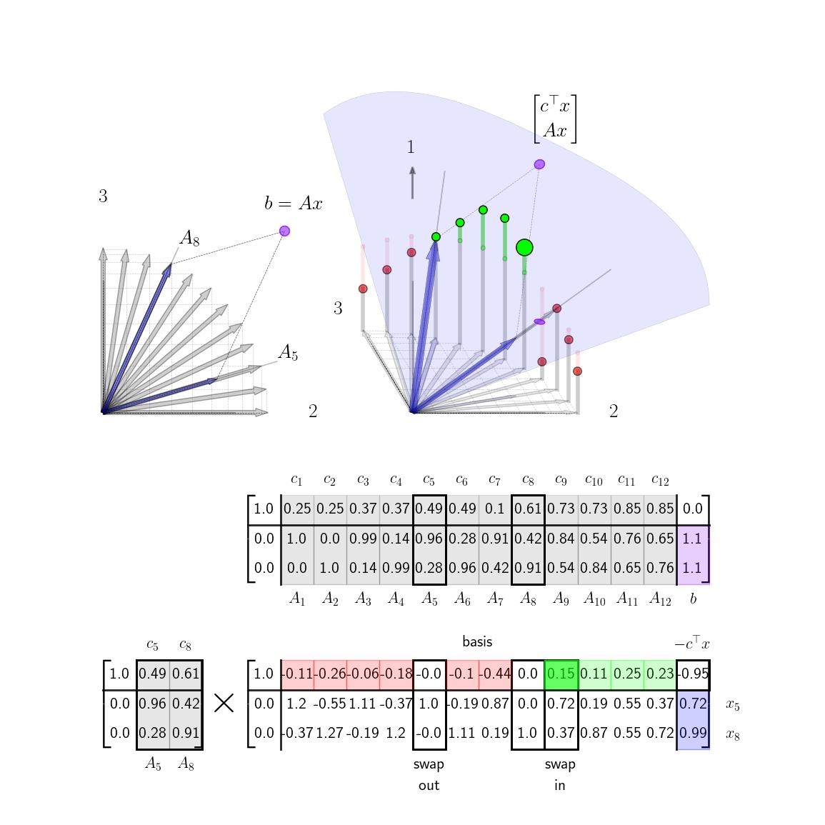
Column Geometry

We now turn to the column geometry of the basic canonical form. For the majority of this post, we will take \(m = 2\) (two rows) and \(n = 12\) (twelve columns). We will choose \(c\), \(A\), and \(b\) to be as follows given in tableau format below.

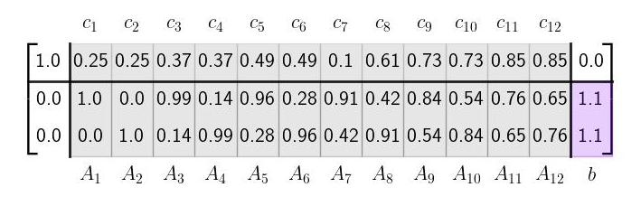
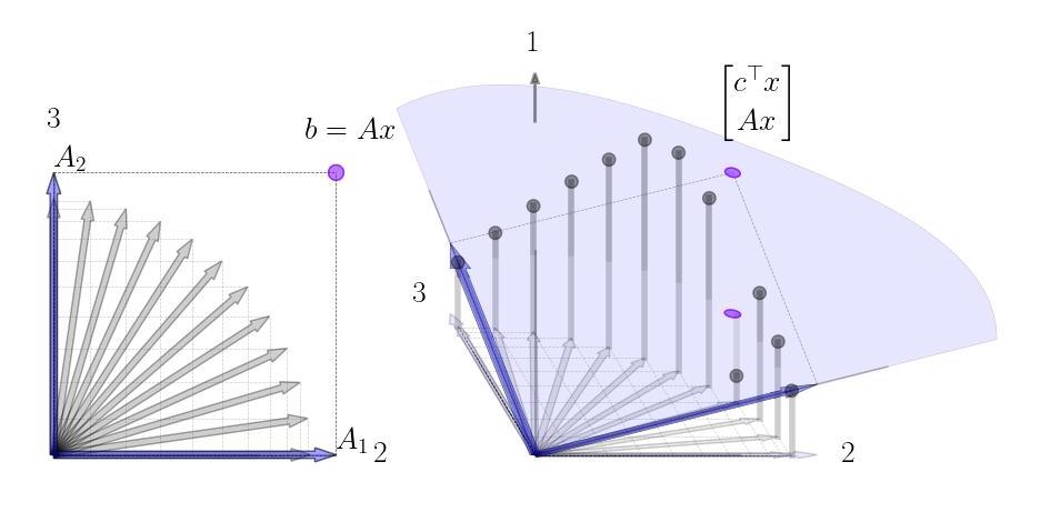
The column geometry of \(A\) and \(b\) is shown here on the left in 2D; the column geometry of the full tableau is shown here on the right in 3D.

Geometry: \(Ax = b\)

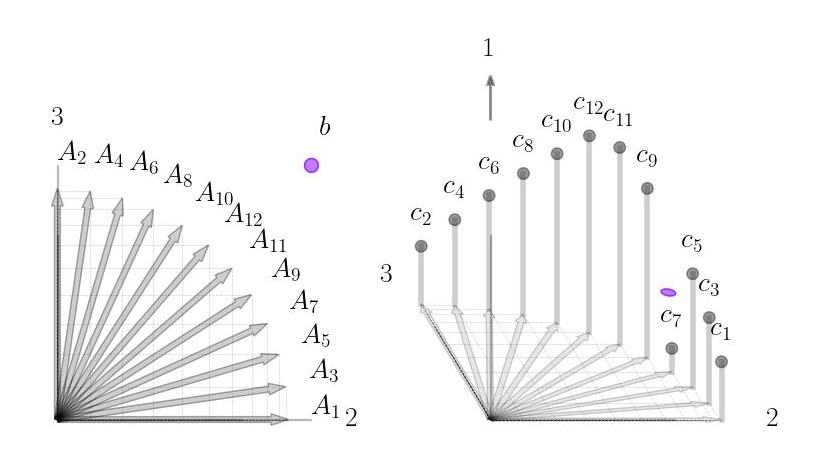
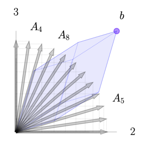
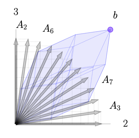
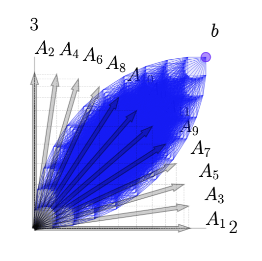
From a column geometry perspective the equality constraint \(Ax = b\) requires that \(x\) be a positive linear combination that constructs \(b\) from the columns of \(A\). We give the basic geometry several examples here.

Note that the fact that \(b \in \mathbb{R}^2\) means that \(x\) will in general have at least two elements that are nonzero. Note that some of these combinations have more positive elements than others. Specifically In each of these cases, we take the minimum norm solution for \(x\) that uses a two, three, four, and then, just for fun, all twelve columns. The coordinates in each case can be visualized by a hypercube of dimension given by the number of nonzero elements. While we can use any number of columns (greater than 2) to construct solutions to \(Ax=b\), we can show, however, that for any optimal value of the linear program there will be an \(x\) that achieves that value with only two (in general \(m\)) non-zero values. Moreover, suppose if we have an optimal \(x\) with more than two nonzero coordinates shifting the mass of \(x\) to any two coordinates that originally had nonzero elements will keep the overall reward the same.

Geometry: Tableu

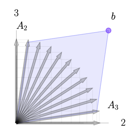
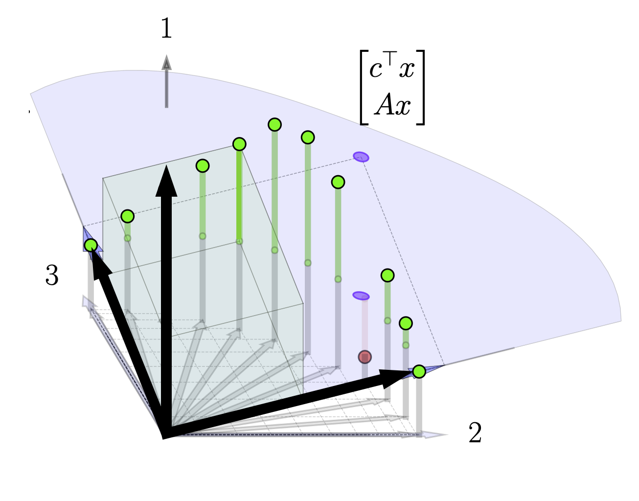
The addition of \(c\) to construct the tableau raises the tips of each column vector \(A_j\) (in a third dimension) to the height of \(c_j\) as illustrated above. For any linear combination \(x\) such that \(Ax = b\), the vector \(\xi = [c^\top x ; \ Ax ]\) will be directly above (or below) the point \(\bar b = [0; \ b]\) in the 3D space. The geometry of this is illustrated here.

Geometrically, then the goal of solving the linear program is to find a positive linear combination of \(x\) such that \(Ax = b\) such that the \(\xi\) is as high above the point \(\bar b\) as possible, ie. to maximize \(c^\top x\). From the discussion above, we have that any optimal solution can be reduced to a solution with only two basis vectors and so because of this we will swap basis vectors in and out in order to increase the height (\(c^\top x \)) until we cannot make any more improvements. In the next section we will get into the details of this method, but here we suggest the reader take a brief look at the animated visualization at the top (or the same visualization lower down) to get a feel for how the algorithm progresses geometrically. Note how the height of \(\xi\) continuously increases and how at the algorithms termination there are no more basis vectors we can swap in that will increase this height.

Prequesites: Gaussian Elimination/Row-Reduction

The operations in the simplex method require basic knowledge of Gaussian elimination and row reduction. A precise understand also requires understanding elementary matrices and how they can be used to perform row operations. For a longer discussion of Gaussian elimination and the column geometry of row operations we refer the reader to this link: Gaussian Elimination: Column Geometry.

Here, we simply note that when we row-reduce a matrix from \(M\) to \(M'\), we are implicitly constructing a sequence of elementary matrices \(E_K,\dots,E_1\) with \(E_k \in \mathbb{R}^{ m \times m}\) such that $$ EM = M' $$ where \(E = E_K\cdots E_1\). Note that as elementary matrices, each individual \(E_k\) is easily invertible and thus we can compute as we go \(E^{-1} = E_1^{-1}\cdots E_K^{-1}\). This allows us to immediately write the above equation as $$ \begin{aligned} M & = E^{-1}EM \\ & = E^{-1}M' = \begin{bmatrix} E^{-1}M_1' & \cdots & E^{-1}M_n' \end{bmatrix} \end{aligned} $$ As shown in this second expansion, here we are writing each column of \(M_j\) as a set of coordinates \(M_j'\) relative to the new basis \(E^{-1}\), ie. row reduction can be seen as changing the basis with respect to which the columns of \(M\) are represented.

Simplex Method: Main Algorithm

We now discuss the three steps of the simplex method. These steps center around row reduction operations which implicitly adjusts the basis we are considering for the columns of \(A\). We note that we will assume that we start with an initial feasible solution that satisfies \(Ax=b\) and \(x\geq 0\). Constructing this initial feasible solution can be done by using an expanded initial tableau. Starting from this initial solution we perform these three operations.

Step 1: Row Reduce Basis Columns

As we perform row operations during the simplex method, we will be implicitly adjusting the basis \(E^{-1}\); specifically the specific row operations will amount to swapping different columns of the tableau into the basis matrix \(E^{-1}\) and representing the rest of the columns with respect to that basis. To illustrate, this we show the tableau at two different steps: the initial two basis vectors columns 1 and 2 and then at the step where the basis vectors are columns 5 and 8. We explicitly show the basis matrix \(E^{-1}\) in each case as well.

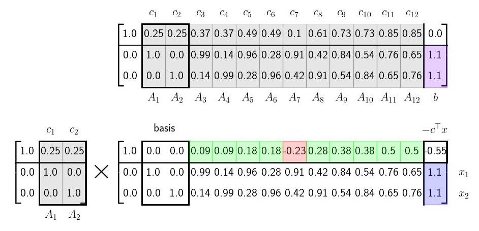
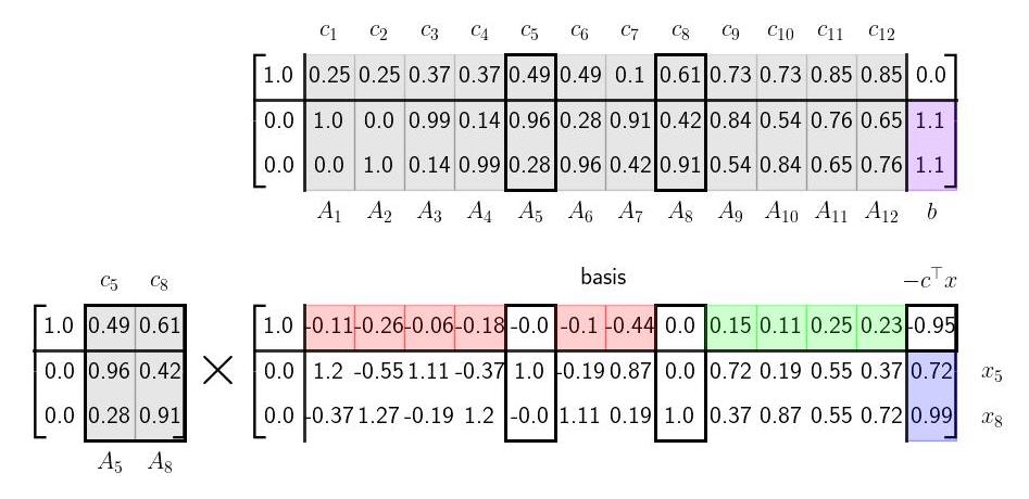
Note how the current two basis columns from the original tableau show up as the last two columns of the basis matrix. The reader is encouraged to check that each column in the original tableau is indeed the column in the updated tableau times the basis matrix.

To be explicit, if we perform row operations so that the \(j\)th and \(j'\)th columns of the tableau are zeros in the top row with an identity below them, then the basis matrix \(E^{-1}\) will have the form below. $$ \begin{aligned} E^{-1} = \begin{bmatrix} 1 & \bar{c}^\top \\ 0 & \bar{A} \end{bmatrix}, \qquad \text{with} \quad \bar{A} = \begin{bmatrix} | & | \\ A_{j} & A_{j'} \\ | & | \end{bmatrix}, \ \bar{c}^\top = \begin{bmatrix} c_j & c_{j'} \end{bmatrix} \quad \text{with} \quad \bar{x} = \begin{bmatrix} x_j \\ x_{j'} \end{bmatrix} \end{aligned} $$ One can easily check that the matrix \(E\) (all the combined row operations performed thus far) can be written as $$ \begin{aligned} E^{-1} = \begin{bmatrix} 1 & \bar{c}^\top \\ 0 & \bar{A} \end{bmatrix}, \qquad \Rightarrow \qquad E = \begin{bmatrix} 1 & -\bar{c}^\top \bar{A}^{-1} \\ 0 & \bar{A}^{-1} \end{bmatrix} \end{aligned} $$ Since all the other elements of \(x\) are 0, we can write \(c^\top x = \bar{c}^\top \bar{x}\) and also \(Ax = \bar{A}\bar{x} = b\). Assuming \(\bar{A}\) is invertible, we can compute explicitly that \(\bar{x} = \bar{A}^{-1}b\). We then have that the last column of the tableau at the current step is given by $$ \begin{aligned} E \begin{bmatrix} 0 \\ b \end{bmatrix} = \begin{bmatrix} 1 & -\bar{c}^\top \bar{A}^{-1} \\ 0 & \bar{A}^{-1} \end{bmatrix} \begin{bmatrix} 0 \\ b \end{bmatrix} = \begin{bmatrix} -\bar{c}^\top \bar{A}^{-1}b \\ \bar{A}^{-1} b \end{bmatrix} = \begin{bmatrix} -\bar{c}^\top \bar{x} \\ \bar{x} \end{bmatrix} = \begin{bmatrix} -c^\top x \\ \bar{x} \end{bmatrix} \end{aligned} $$ We now see that as we perform row operations to select different basis columns, the last column of the tableau shows us both the current nonzero elements of our current guess for \(x\) as well as (minus) the current objective value.

Step 2: Selecting next basis columns to swap in

From the above discussion, we see that row reducing two basis columns of the tableau to 0's in the top row and an identity (possibly with the columns rearranged) in the bottom two rows allows us to track our current estimate of \(x\) and the current value of the objective function at that \(x\). From here, we could simply check the objective value at all pairs of basis columns and see which pair gives us the largest value. This combinatorially procedure is of course not tractable, but fortunately we will be able to use the tableau information also to tell us which columns we should swap in to improve the objective value.

Noting the structure of \(E^{-1}\), we see that the first column is the first standard basis vector and thus the top row of the tableau corresponds to the height above the plane generated by the basis columns. We illustrate this here. Note the three basis vectors shown - the first standard basis vector and the two columns of the original tableau. Each column of the current tableau is the coordinates of the that original tableau column relative to the current basis. Specifically, note that if the first element of these coordinates (the top element) is positive that column in the original tableau is above the plane spanned by the current two basis columns; if it is negative it is below this plane. We illustrate this for two different columns here.

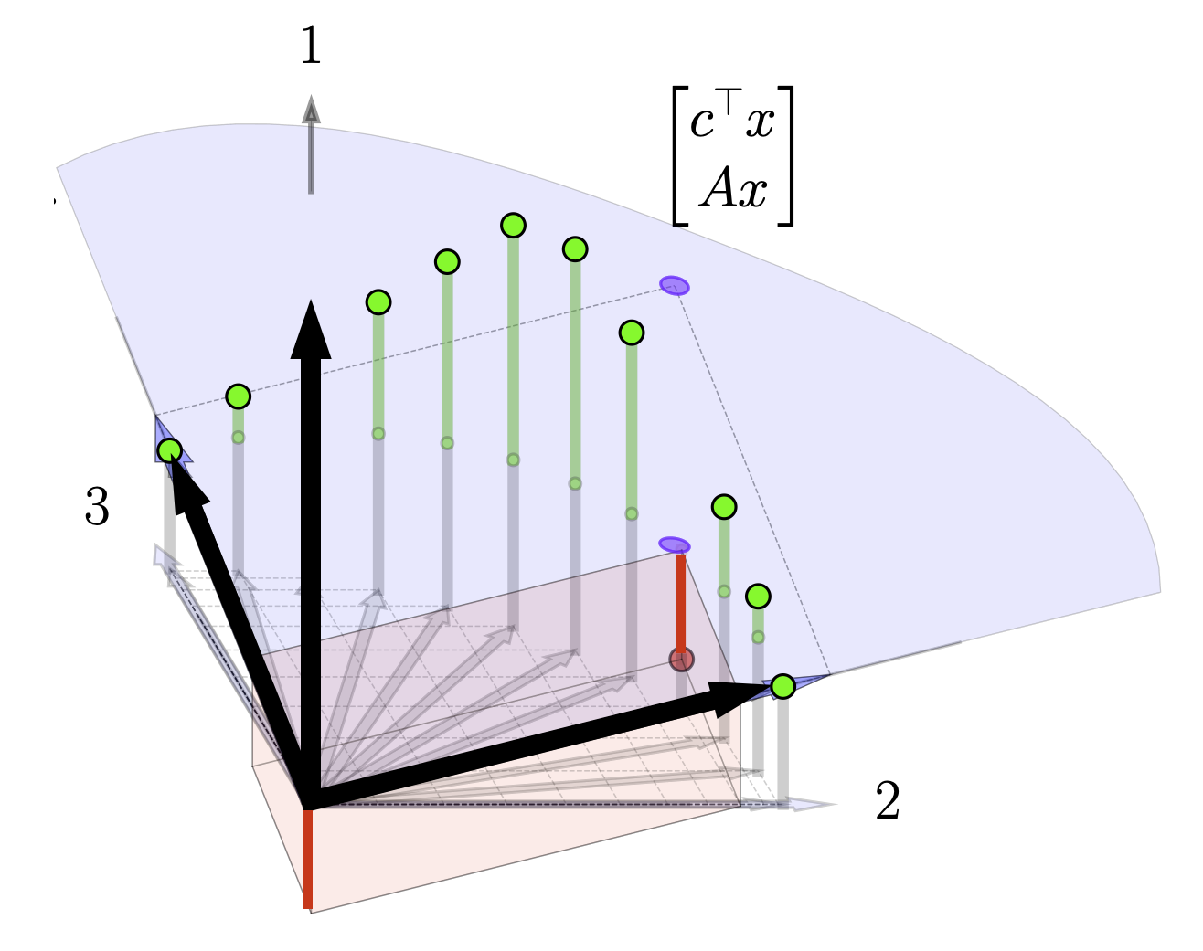
This fact gives us a procedure for swapping in basis columns. At each pivot step; we pick a non basis column to swap in with a positive element in the top row, ie. a column that is above the current basis plane. Swapping in this new basis column will raise the plane and thus increase our objective function. If there is more than one positive element in the top row, our choice is somewhat arbitrary. There are several entering variable rules that can be applied such as Devex algorithm. In our examples below, we make a somewhat contrived choice so that the objective function will change slowly in order to visualize the mechanics of the procedure. In reality, in the below example, we can actually just take one or two quick steps to the solution by picking the later basis columns. In more complicated settings where the costs weren't selected for visualization purposes it may be less clear which basis columns to swap in. If there are no columns with positive elements in the top row at any given step, than we're done and our current basis vectors are optimal. Below we show the tableau in process at an intermediate step where we select a basis vector to swap in.

Step 3: Choosing basis column to swap out

We are now left with a question of which basis vector to swap out at each step. Intuitively, we swap in basis vectors in order to raise the height of the basis plane. We choose which vector to swap out in order to ensure that that we can still construct \(b\) as a positive combination of the two basis vectors. In the graphic depiction above this corresponds to swapping out the current basis vector that is on the same side of the solution as the new basis vector so that the vector \(b\) always lies between the current basis columns of \(A\). If we were to select basis columns that were on the same side of \(b\) and solutions to \(Ax =b\) would involve negative elements in \(x\) as illustrated here. For higher dimensional problems, we always want to main that \(b\) is inside the \(m\)-dimensional cone of positive combinations of the \(m\) basis vectors. Algebraically, the way we ensure this condition as by looking at elements of the columns of the lower columns of the tableau. Specifically, if we are swapping in the \(k\)th column, we need to row reduce \(A'_k\) to some column of the identity (and then swap out that current basis column). We need to make sure that our current estimate of \bar{x} stays positive so we care about how these row operations affect the last column of the tableau, b', as well. If we choose the \(\ell\)th column of the identity, we get the following reduction steps shown here on column \(k\)th column and the last column. $$ \begin{aligned} \begin{bmatrix} A'_{1k} & b'_1\\ \vdots & \vdots\\ A'_{\ell k} & b'_\ell \\ \vdots & \vdots \\ A'_{mk} & b'_m \end{bmatrix} \rightarrow \begin{matrix} \text{row} \\ \text{reduction...} \end{matrix} \rightarrow \begin{bmatrix} 0 & b'_1 - (A'_{1k}b'_\ell/A'_{\ell k})\\ \vdots & \vdots\\ 1 & (b'_\ell /A'_{\ell k})\\ \vdots & \vdots \\ 0 & b'_m - (A'_{mk}b'_\ell/A'_{\ell k}) \end{bmatrix} \end{aligned} $$ Note that each element of \(b'\) will be positive (since we ensured that on the last step). Next note that we must pick a row \(\ell\) such that \(A'_{\ell k}\) is positive (so that \((b'_\ell/A'_{\ell k})\) will be positive as well.) (If there is no such row than the problem is unbounded and there is no solution.) For the remaining entries, we can safely ignore any rows such that \(A'_{ik}\) is negative since then \(b'_i - (A'_{ik} b'_\ell/A'_{\ell k})\) is guaranteed to be positive. We are then left with the condition that we need to choose row \(\ell\) such that $$ b'_i - A'_{ik}b'_{\ell}/A'_{\ell k} > 0 $$ for all \(i \neq \ell \) such that \(A'_{ik}>0\). Choosing \(\ell\) to be the row where the fraction \(b'_i/A'_{\ell k}\) is minimized accomplishes this.

In the above example note, that as we swap in column 9, we have a choice of swapping out either column 5 or column 8. We have that \(A'_9 = [ 0.7 ; 0.4] \). Since both elements are positive, we can consider swapping both of them out. Computing the fractions detailed above we have that \(b'_1/A'_{1,9} = 0.72/0.72 = 1.\) and \(b'_2/A'_{2,9} = 0.99/0.37= 2.68\) and so we have that we should swap out column 5 (since it has a 1. in the appropriate row). From the image note that column 5 is indeed on the same side of the target point \(b\), so when we make the swap \(b\) will still lie inbetween the basis columns.

Visualization

We now visualize the full algorithm in action starting from the initial basis