Algebraic graph theory is a powerful mathematical discipline that derives matrices from graphs, studies their linear algebraic properties, and then applies those insights to graph problems. It has become a must-know area of mathematics for many subdisciplines of optimization and machine learning such as Markov decision processes, reinforcement-learning, path-planning, and commodity optimization. In this post, we detail a fundamental decomposition result for the well-known node-edge incidence matrix of a graph.

Basic Graph Setup

A graph \(\mathcal{G}=(\mathcal{V},\mathcal{E})\) is a mathematical object consisting of discrete states (referred to as nodes or vertices) \(\mathcal{V}\) and a connectivity structure between them, ie. a set of edges \(\mathcal{E}\). We will focus mostly on directed graphs, ie. graphs where each edge has an orientation "from one node to another node". In many optimization problems involving graphs, we will be considered with variables that take values on either each edge or each node. For example, in many routing or flow optimization problems, we will define a vector \(x \in \mathbb{R}^{|\mathcal{E}|}\) where each \(x_j\) is the amount of mass or flow on edge \(j \in \mathcal{E}\). Often \(x\) will represent the indicator vector for a path or flow distribution of some commodity. We illustrate one such vector \(x\) in the figure below. On the other hand, we will also often want to define variables on the nodes \(v \in \mathbb{R}^{|\mathcal{V}|}\) where \(v_i\) is a value on node \(i \in \mathcal{V}\). \(v_i\) can be thought of as the ``height'' of that node illustrated in the figure below as well. In physics problems, \(v\) often corresponds to heights, voltages, or some other potential energy indicator. In flow optimization problems, often \(v\) represents some cost-to-go measure from that node to the sink.

Node-Edge Incidence Matrix

Algebraic graph theory defines many types of matrices for each graph, but perhaps the most fundamental is the node-edge incidence matrix that we will call \(E \in \mathbb{R}^{|\mathcal{V}|\times |\mathcal{E}|}\). $$ \begin{aligned} E_{ij} = \begin{cases} -1 & \text{ if edge \(j\) starts at node \(i\) } \\ 1 & \text{ if edge \(j\) ends at node \(i\) } \\ 0 & \text{ otherwise} \end{cases}, \end{aligned} $$ Each row corresponds to a node and each column corresponds to an edge. The row for each node contains a -1 if the edge comes out of the node, a 1 if the edge goes into that node, and a 0 otherwise.

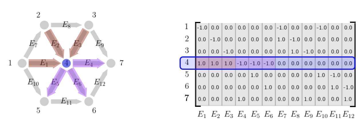
Equivalently, the column for each edge contains -1 for the node the edge starts from and a 1 for the node the edge ends at and a 0 otherwise.

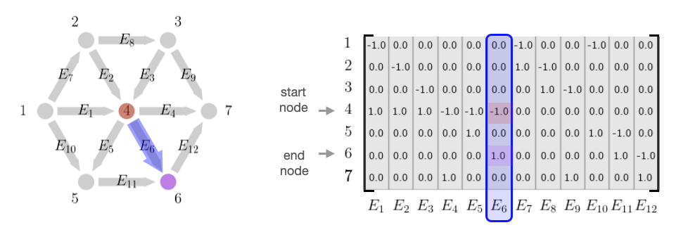
Each row of the incidence matrix represents a mass conservation equation at that particular node and as a result, for flow optimization problems we often use constraints of the form shown below where \(S \in \mathbb{R}^{|\mathcal{E}|}\) is a source-sink vector that has the same form as a column of the incidence matrix and indicates the node the flow starts from (the source) and the node the flow goes to (the sink). This incidence matrix shows up in many physica equations (circuit balances, etc) and many optimization problems especially those focused on flow using the above constraint (shortest path optimization, commodity flow optimization, etc). Extensions of it are also form the foundation for Markov decision process analysis.

Spanning Trees & Cycles

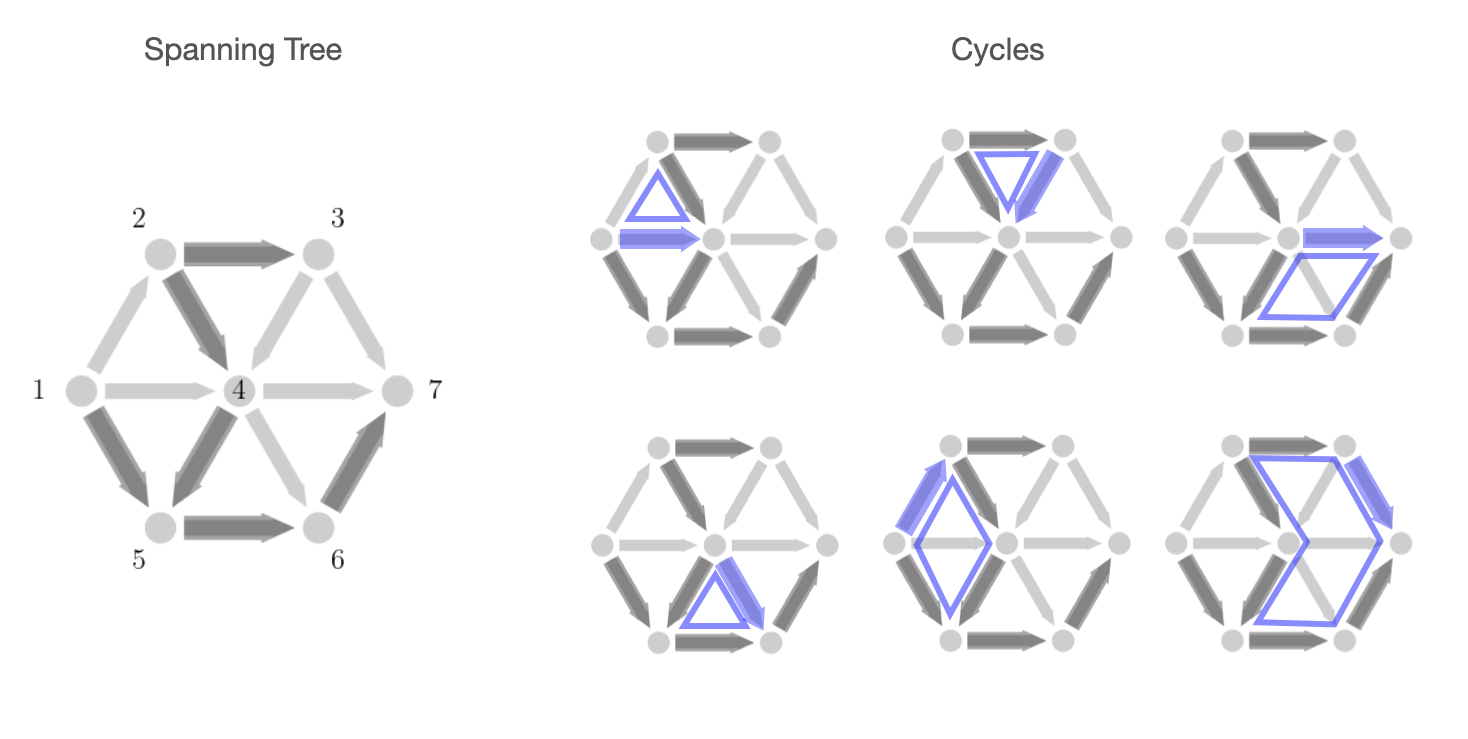
In a moment we will introduce a decomposition of incidence matrices that is based on the ideas of trees and cycles of a graph. For a completely connected graph, a spanning tree is a subset of the edges of a graph that connect all the nodes without forming any cycles. Because of this, each spanning tree has exactly \(\mathcal{V}-1\) edges, one less than the number of nodes. Every other edge that is not in the spanning tree corresponds to a specific cycle of the graph that can be formed by taking that edge along with other edges in the spanning tree. The spanning tree essentially already contains all the edges of that the cycle and the non-spanning tree edge is the edge left out. It can also be shown that the set of cycles corresponding to each of the non-spanning tree edges forms a linearly independent set and actually a basis for the full cycle space. (More details in the nullspace section below.) We illustrate these cycles here given a spanning tree of the graph shown.

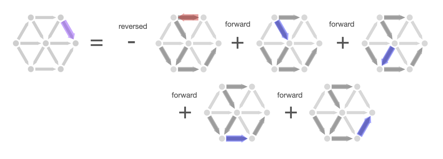
This cycle idea also allows us to construct any non-spanning tree edge as a linear combination of spanning tree edges. In particular, to get from the start node to the end node of the non-spanning tree edge, we could simply traverse the edge or we could walk the other way around the cycle using edges in the spanning tree to have the same effect. Algebraically, this is equivalent to constructing a column of the incidence (not in the spanning tree) from other columns (in the spanning tree) by taking a linear combination with 1's and -1's. We add the column if we are traversing the edge along it's orientation; we subtract the column if we are traversing the edge in the opposite direction.

Tree-Cycle Decomposition

From the above discussion, we have that we can decompose graph incidence matrices in the following way. For a fully connected graph, we can write $$ \begin{aligned} E = T\Big[ \ I \ \ M \ \Big] = \Big[ \ T \ \ TM \ \Big] \end{aligned} $$ Here \(T \in \mathbb{R}^{|\mathcal{V} \times \mathcal{V}-1|}\) is the incidence matrix for a spanning tree and \(M\) is a matrix related to the cycles. Explicitly, each column of \(M\) corresponds to a linear combination of spanning tree edges that constructs an edge not in the spanning tree. Note here that the dimensions of \(T\) are fixed since spanning trees must always have one less edge than the number of nodes. Note also that for ease of notation, we have assumed that the first \(\mathcal{V}-1\) edges of the graph form the spanning tree. If this is not the case, the identity matrix in the above form will be shuffled throughout the \(M\) matrix. (This corresponds to a simple reordering of the edges so we can assume the above form without loss of generality.) We illustrate the structure of this decomposition according to the tree and cycles as discussed above here.

In the general case when the graph may not be full connected, this expansion becomes $$ \begin{aligned} E = \underbrace{ \begin{bmatrix}p T_1 & \cdots & 0 \\ \vdots & \ddots & \vdots \\ 0 & \cdots & T_k \end{bmatrix}}_{F} \begin{bmatrix} I & \cdots & 0 & M_1 & \cdots & 0\\ \vdots & \ddots & \vdots & \vdots & \ddots & \vdots \\ 0 & \cdots & I & 0 & \cdots & M_k \end{bmatrix} \end{aligned} $$ where \(F\) is the incidence matrix for what is called a spanning forest (a set of spanning trees) where each tree corresponds to one of the \(k\) connected components, that gives the block diagonal structure.

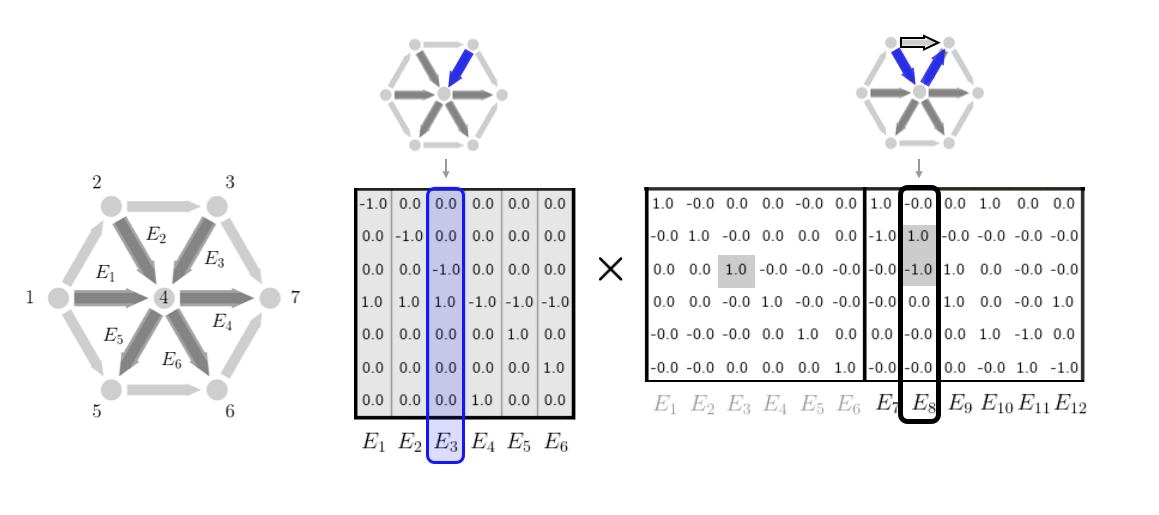
We give two examples of this decomposition spelled out in detail with images.

Example 1: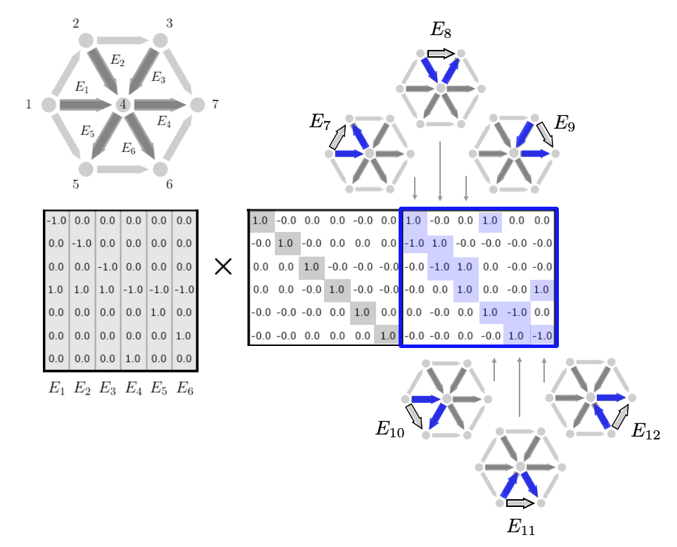

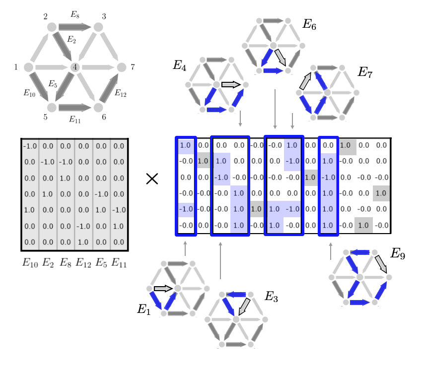
Example 2:

Fundamental Subspaces

The above construction gives a clear picture of each of the four fundamental subspaces for the incidence matrix and their interpretation in terms of edge flows and potential values. We detail each of the here

Range of \(E\): Total mass in and out of nodes

Taking linear combinations of the columns of \(E\) gives a vector in \(\mathbb{R}^{|\mathcal{V}|}\). For a particular edge flow \(x\), each element of \(Ex\) is the flow in that node minus the flow out, ie. the total mass in or out of the node depending on the sign.

Nullspace of \(E\): Cycle Flow Space

The nullspace is defined by the equation \(Ex=0\). This corresponds to an edge flow vector that conserves mass at each node which intuitively corresponds to cyclic flows in the graph. The above decomposition allows us to make this explicit. Specifically, we can write a basis for the nullspace as $$ \begin{aligned} C = \begin{bmatrix} -M \\ I \end{bmatrix} \end{aligned} $$ Multiplying out we can see immediately that \(EC = T(-M + M) = 0\). Furthermore, we have that each column of \(C\) is linearly independent because of the identity in the bottom half. Rigorously, this is because $$ \begin{aligned} Cz = 0 \implies \begin{bmatrix} Mz \\ z \end{bmatrix} = \begin{bmatrix} 0 \\ 0 \end{bmatrix} \implies z = 0 \end{aligned} $$ which is the definition of linear independence. A slightly longer argument shows that \(C\) spans the nullspace of \(E\) as well. Rigorously, any \(x\) such that \(Ex=0\) can be written as \(x = Cz\) since we can decompose \(x\) as \(x = [x' ; x'']\) and write $$ \begin{aligned} 0 = Ex = T(x' + M x'') & \implies x' + M x'' = 0 \\ & \implies x' = -M x'' \\ & \implies x = \begin{bmatrix} -M \\ I \end{bmatrix} x'' \\ & \implies x = Cz \end{aligned} $$ with \(z = x''\). Note that in the middle step we have used the fact that the columns of \(T\) are linearly independent. We thus have that the columns of \(C\) each indicator vectors for a cycle of the graph form a basis for the nullspace of \(E\). Any other flow where mass is conserved can be written as a linear combination of these cycles.

Nullspace of \(E^\top\): Constant Node Heights

Note that each column of the incidence matrix sums to 0 and thus the left nullspace or nullspace of \(E^\top\) is given by any constant vector, such as the vector of all 1's. Relative to the flow variables this implies that \(\mathbf{1}^\top Ex =0\) for any \(x\), ie. any vector of the form \(Ex\) has the same of amount of entering and exiting the network. Relative to the node variables, left multiplying by any node variable \(v\), \(v^\top E\) is independent of any constant shift of \(v\).

Range of \(E^\top\): Edge Tension Space:

Lastly, any linear combination of the rows of the form \(v^\top E\) gives the relative difference along the edges for different node potential values. As discussed in the previous section, this is independent of any constant shift.