For a \(2 \times 2 \) matrix, we can expound on the eigenstructure precisely. This is useful for \(2 \times 2\) matrices specifically but it is also useful for getting intuition for matrices in general.
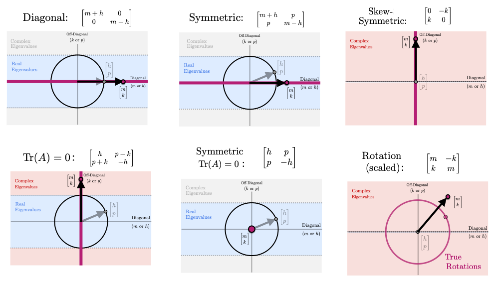
For the following, we will discuss the \( 2 \times 2 \) matrix $$ A = \begin{bmatrix} a & b \\ c & d \end{bmatrix} = \begin{bmatrix} | & | \\ A_1 & A_2 \\ | & | \end{bmatrix} = \begin{bmatrix} - & \bar{A}_1^T & - \\ - & \bar{A}_2^T & - \end{bmatrix} $$ Another way to represent \(A\) that will prove useful is $$ A = \begin{bmatrix} m + h & p -k \\ p + k & m - h \end{bmatrix} $$ where $$ m = \tfrac{1}{2}\big(a+d), \quad h = \tfrac{1}{2}\big(a-d), \qquad p = \tfrac{1}{2}\big(b+c), \quad k = h = \tfrac{1}{2}\big(c-b) $$ Note that here \(m\) and \(p\) are the averages of the diagonal and off-diagonal elements (respectively) and \(h\) and \(k\) are the differences. This \(mhpk\)-parametrization is particularly useful for considering limiting cases or special types of matrices. We detail some of these in the image below. Only \(m \neq 0 \) is a scaled identity matrix; \(m,h,p \neq 0\) is symmetric. only \(k \neq 0\) is skew symmetric; only \(m,k \neq 0\) is a scaled rotation; \(h,p\neq 0\) is symmetric with zero trace. (This parametrization also suggests other interesting categories of \(2 \times 2\) matrices such as \(m,p \neq 0\) (symmetric matrices with constant diagonal) or \(h,k \neq 0\) (a zero-trace matrix) that has some rotation like properties.) We comment also that this parametrization suggests several matrix decompositions. Specifically, we will consider $$ A = \begin{bmatrix} m & -k \\ k & m \end{bmatrix} + \begin{bmatrix} h & p \\ p & -h \end{bmatrix} $$ Here we've decomposed \(A\) into two orthogonal matrices. the first is a scaled rotation and the second is a symmetric zero-trace matrix that turns out to be a scaled reflection.
The determinant of \( A \) will also prove important. $$ det(A) = ad - bc = m^2 - h^2 - p^2 + k^2 $$ We also can note the inverse of \(A\) $$ A^{-1} = \frac{1}{det(A)} \begin{bmatrix} d & -b \\ -c & a \end{bmatrix} = \frac{1}{det(A)} \begin{bmatrix} m - h & -p + k \\ -p - k & m + h \end{bmatrix} $$
The characteristic polynomial of the matrix is given by $$ char_A(s) = s^2 - (a+d)s + (ad - bc) = s^2 - tr(A) + det(A) $$ Note in the \(mhpk\)-parametrization this becomes $$ char_A(s) = s^2 - 2ms + m^2 - h^2 - p^2 + k^2 $$ The eigenvalues are then given by the roots of the characteristic polynomial which in this case can be computed using the quadratic equation. $$ \lambda_{1,2} = \tfrac{1}{2}tr(A) \pm \sqrt{\left(\tfrac{tr(A)}{2}\right)^2 -det(A) } $$ $$ \lambda_{1,2} = \tfrac{a+d}{2} \pm \sqrt{\left(\tfrac{a+d}{2}\right)^2 -ad-bc } $$ $$ \lambda_{1,2} = m \pm \sqrt{h^2+p^2 - k^2} $$ This last formula specifically gives us some direct insight into the structure of the eigenvalues. Below we list these ideas and also whatever generalizations there are to \(n \times n\) matrices. First, the two eigenvalues are centered around \(m\) which is the trace divided by 2 or the arithmetic mean of the diagonal. This extends to the \(n \times n\); the arithmetic mean of the diagonal (ie. \(tr(A)/n\)) is the centroid of the eigenvalues. Secondly, the geometry of the vectors $$ u_\pm = \begin{bmatrix} m \\ \pm k \end{bmatrix}, \qquad v_\pm = \begin{bmatrix} \pm h \\ p \end{bmatrix}, $$ tell us a lot about the matrix and it's eigenvalues. For a symmetric matrix (\(k=0\) ) the eigenvalues are given by $$ \lambda_{1,2} = m \pm \sqrt{h^2+p^2} = m \pm \left|\left|\begin{bmatrix} h \\ p \end{bmatrix}\right| \right|_2 $$ In this case, the definitiness of the matrix is determined by the relative size of \(m\) with the norm of \(v\). A symmetric \(2\times 2\) matrix is definite if and only if $$ |m| > \left|\left|\begin{bmatrix} h \\ p \end{bmatrix}\right| \right|_2 $$ Positive or negative definite depends on the sign of \(m\). The discrimant is given by $$ p^2 + h^2 - k^2 = \left|\left|\begin{bmatrix} h \\ p \end{bmatrix}\right| \right|_2^2 - k^2 $$ \(A\) has real eigenvalues if and only if $$ |k| \leq \left|\left|\begin{bmatrix} h \\ p \end{bmatrix}\right| \right|_2 $$ If \(p=h=0\), then the eigenvalues are given by $$ \lambda_{1,2} = m \pm k i = \sqrt{m^2 + k^2} e^{\pm i\phi} $$ with \(\phi = tan^{-1}\left(\tfrac{k}{m}\right)\) where the second equality gives the polar form. This last characterization shows a close relationship between a matrix of the form $$ A = \begin{bmatrix} m & -k \\ k & m \end{bmatrix} = \sqrt{m^2 + k^2} \begin{bmatrix} \tfrac{m}{\sqrt{m^2 + k^2}} & -\tfrac{k}{\sqrt{m^2 + k^2}} \\ \tfrac{k}{\sqrt{m^2 + k^2}} & \tfrac{m}{\sqrt{m^2 + k^2}} \end{bmatrix} = \sqrt{m^2 + k^2} \begin{bmatrix} \cos(\phi) & -\sin(\phi) \\ \sin(\phi) & \cos(\phi) \end{bmatrix} $$ and the complex conjugate pair \(m \pm ki \). Indeed much of the intuition behind complex eigenvalues is grounded in understanding matrices of this form. Note that the last two equalites write the matrix as a scaled rotation closely related to the polar form of the eigenvalues.
From the above analysis, it seems profitable to plot \(u_\pm \) and \(v_\pm \) in a 2D space analogous to the complex plane. For \(v_\pm = 0\) this space is precisely a picture of the complex plane and the vectors u_\pm are the eigenvalues of the matrix. When \(v_\pm \neq 0\) we can modify the picture in the following way. Plot the vector \(v_\pm \) and the ball it touches. Properties of the eigenvalues of \(A\) are then given by what region \(u_\pm\) falls in relative to the ball generated by \(v_\pm\). These regions are shown in the diagram below

We also give several specific examples of different types of matrices to explore this visualization further.

While the above eigenvalue analysis is insightful, we must also consider the eigenvectors in order to get a full picture of the action of a matrix. We will discuss primarily discuss right eigenvectors here, but analogous results apply to left eigenvectors as well.
For an eigenvalue \(\lambda\), the right eigenvector is contained in the nullspace of $$ \lambda I-A = \begin{bmatrix} \lambda - a & -b \\ -c & \lambda - d \end{bmatrix} $$ Row-reducing this matrix gives $$ \underbrace{ \begin{bmatrix} 1 & 0 \\ c & 1 \end{bmatrix} }_{E_2} \underbrace{ \begin{bmatrix} \tfrac{1}{\lambda-a} & 0 \\ 0 & 1 \end{bmatrix} }_{E_1} \begin{bmatrix} \lambda - a & -b \\ -c & \lambda - d \end{bmatrix} = \begin{bmatrix} 1 & -\tfrac{b}{\lambda - a} \\ 0 & \tfrac{(\lambda - d)(\lambda-a)-cb}{\lambda - a} \end{bmatrix} = \begin{bmatrix} 1 & -\tfrac{b}{\lambda - a} \\ 0 & 0 \end{bmatrix} $$ where the last equation is from \(\lambda\) being a root of the characteristic polynomial. We then have the following two characterizations of a right eigenvector for \(\lambda\). $$ V_{1,2} \sim \begin{bmatrix} b \\ \lambda_{1,2} - a \end{bmatrix} \sim \begin{bmatrix} \lambda_{1,2} - d \\ c \end{bmatrix} $$ The first characterization here comes from the row reduction done above (where the \(1,1\) entry of the matrix is taken as the pivot); the second characterization comes from if the \(2,2\) entry of the matrix is taken as the pivot. We note also that each of these vectors is clearly orthogonal to one of the rows of the matrix above Since in a rank-1 \(2 \times 2 \) matrix the rows are just scalings of each other, being orthogonal to one row is the same as being orthogonal to other other so we could have have just read off both of these characterizations initially. (Again, note that this rank-1 condition (and thus the above eigenvector characterization) is not true for all \(\lambda\) but only when \(\lambda\) satisfies the characteristic equation.)
Along with picking vectors orthogonal to both (in this case, either) row, there is another way to read off eigenvectors based on diagonalizing \( \lambda I-A\). If we diagonalize \( \lambda I - A\) we get $$ \lambda I - A = \begin{bmatrix} \lambda - a & - b \\ -c & \lambda - d \end{bmatrix} = \begin{bmatrix} | & | \\ V_1 & V_2 \\ | & | \end{bmatrix} \begin{bmatrix} \lambda - \lambda_1 & 0 \\ 0 & \lambda - \lambda_2 \end{bmatrix} \underbrace{ \begin{bmatrix} -& W_1^T & - \\ -& W_2^T & - \end{bmatrix} }_{V^{-1}} $$ $$ \begin{bmatrix} \lambda - a & - b \\ -c & \lambda - d \end{bmatrix} = \begin{bmatrix} | \\ V_1 \\ | \end{bmatrix} (\lambda-\lambda_1) \begin{bmatrix} - & W_1^T & - \end{bmatrix} + \begin{bmatrix} | \\ V_2 \\ | \end{bmatrix} (\lambda-\lambda_2) \begin{bmatrix} -& W_2^T & - \end{bmatrix} $$ If we plug in \(\lambda_2\), then the second matrix term in the sum goes to 0 and we get that both columns of the resulting matrix are actually scalings of \(V_1\). Similarly if we plug in \(\lambda_1\), then the columns become scalings of \(V_2\) From this we have that $$ V_1 \sim \begin{bmatrix} \lambda_2 - a \\ -c \end{bmatrix} \sim \begin{bmatrix} -b \\ \lambda_2 - d \end{bmatrix} $$ and that $$ V_2 \sim \begin{bmatrix} \lambda_1 - a \\ -c \end{bmatrix} \sim \begin{bmatrix} -b \\ \lambda_1 - d \end{bmatrix} $$ Note here that the of the eigenvalues/eigenvectors is opposite as opposed to above where it was the same. Note again that the lengths of of the eigenvectors (for each eigenvalue) here are not the same and one would need to work a little harder to show how they differ. Again each of these different subspace characterizations is only the same because \(\lambda\) is a root of the characteristic polynomial. Any attempt to show that these vectors have the same span will involve using the fact that \((\lambda-a)(\lambda-d)-cb = 0\). The rank of \(\lambda I - A\) dropping and it's relationship to the eigenvectors is given in the following illustration
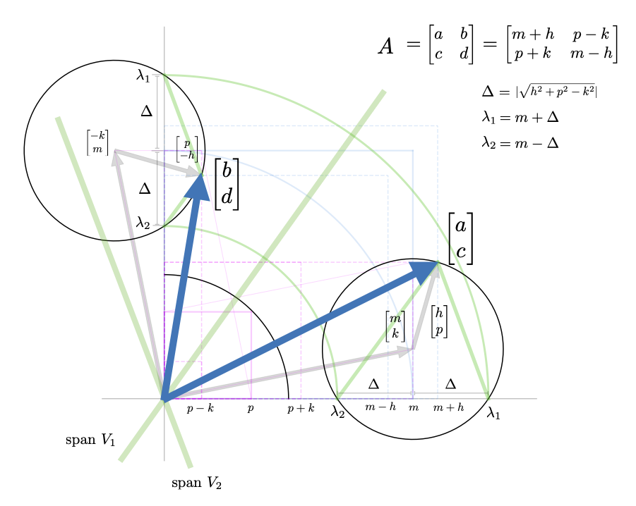
Plugging in the eigenvalues for \(\lambda\) to the above forms gives several specific characterizations. $$ V_{1,2} \sim \begin{bmatrix} b \\ \lambda_{1,2} - a \end{bmatrix} = \begin{bmatrix} p-k \\ -h \end{bmatrix} \pm \begin{bmatrix} 0 \\ \sqrt{p^2+h^2-k^2} \end{bmatrix} $$ $$ V_{1,2} \sim \begin{bmatrix} \lambda_{1,2} - d \\ c \end{bmatrix} = \begin{bmatrix} h \\ p+k \end{bmatrix} \pm \begin{bmatrix} \sqrt{p^2+h^2-k^2} \\ 0 \end{bmatrix} $$ $$ V_1 \sim \begin{bmatrix} \lambda_2 - a \\ -c \end{bmatrix} = \begin{bmatrix} -h \\ -(p+k) \end{bmatrix} - \begin{bmatrix} \sqrt{p^2 + h^2 - k^2} \\ 0 \end{bmatrix} $$ $$ V_1 \sim \begin{bmatrix} -b \\ \lambda_2 - d \end{bmatrix} = \begin{bmatrix} -(p-k) \\ h \end{bmatrix} - \begin{bmatrix} 0 \\ \sqrt{p^2 + h^2 - k^2} \end{bmatrix} $$ $$ V_2 \sim \begin{bmatrix} \lambda_1 - a \\ -c \end{bmatrix} = \begin{bmatrix} -h \\ -(p+k) \end{bmatrix} + \begin{bmatrix} \sqrt{h^2+ p^2 - k^2} \\ 0 \end{bmatrix} $$ $$ V_2 \sim \begin{bmatrix} -b \\ \lambda_1 - d \end{bmatrix} = \begin{bmatrix} -(p-k) \\ h \end{bmatrix} + \begin{bmatrix} 0 \\ \sqrt{h^2+ p^2 - k^2} \end{bmatrix} $$ We also Some of these characterizations are illustrated in the visuals below, but we should also note that \(m\) does not appear in any of the formulas. The reason for this is that \(m\) gets added to both diagonal elements equally and thus provides the component of \(A\) strictly proportional to the identity. $$ A = m \begin{bmatrix} 1 & 0 \\ 0 & 1 \end{bmatrix} + \begin{bmatrix} h & p-k \\ p+k & h \end{bmatrix} $$ Thus for any value of \(m\) the matrix has the same eigenvectors. Since adding a scaling of the identity shifts the eigenvalues but does not change the eigenvectors this is to be expected.
We now suggest a way to visualize the eigenstructure related to the column geometry of a \(2 \times 2\) matrix. This visualization is quite dense and so we will build it up in stages. We first look at the case where both eigenvalues are real.

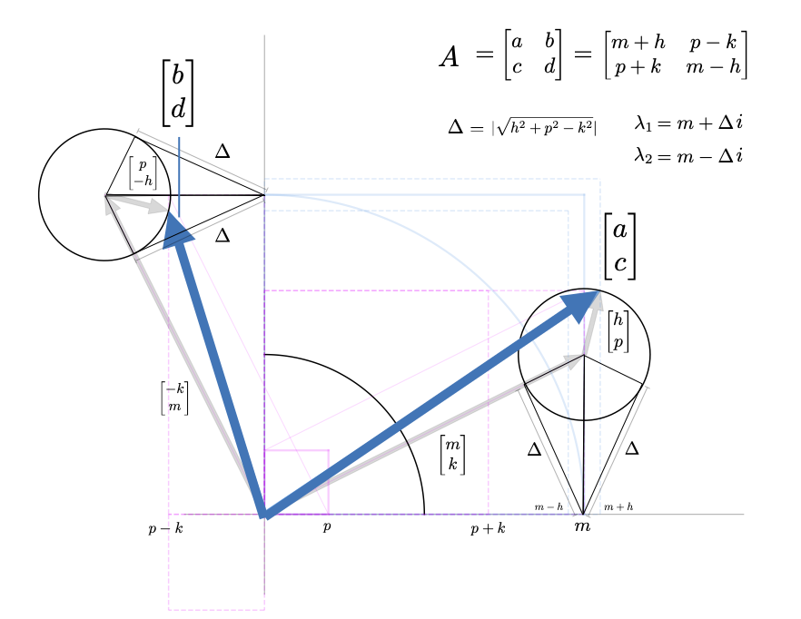
We then consider the case where the eigenvalues are complex.
