When we define a matrix, we define both columns and rows of the matrix. When we think about the geometry of a linear transformation sometimes we focuse on a matrix as a set of columns and sometimes we think of it as a set of rows. These column and row geometries can both be fruitful perspectives and we give more details on each below.
We note that for this discussion we are assuming that a matrix \(A \in \mathbb{R}^{m \times n}\) operators on a column vector \(x \in \mathbb{R}^n \) by left multiplying, \(Ax\). All the intuition we develop would be flipped if we were primarily considering right multiplying row vectors by the matrix \(A\).
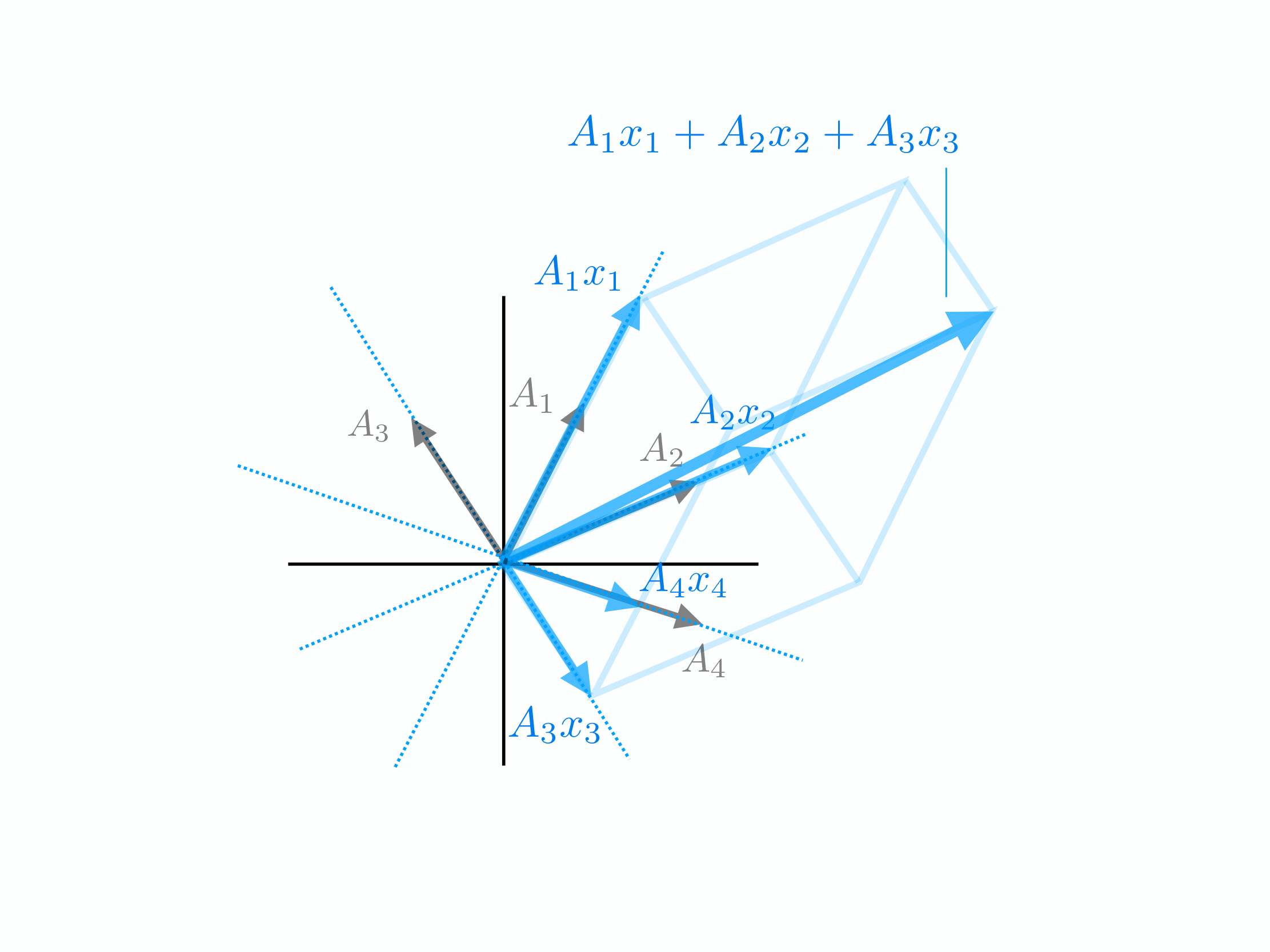
COLUMN GEOMETRYThe column geometry of a matrix is probably the most natural and we have already expounded on it in detail in our previous discussion of linear combinations. When visualizing the column geometry, we represent each columns of a matrix \(A_1, \dots, A_n\) as a vector in the co-domain. Each of these columns defines where a given standard basis vector \(I_1,\dots,I_n\) maps to under the transformation and this in turn defines how the whole space transforms. When we multiply a vector \(x\) by \(A\), \(x\) defines a linear combination of the columns of \(A\) as previously discussed. This picture is continually useful in analysis. We note that from this picture we can easily visualize the subsapce in the co-domain spanned by the columns. This is known as the range. Though it is slightly more complicated, we can also use this geometry to visualize the nullspace of \(A\), ie. the subspace of vectors \(x\) in the domain such that \(Ax =0\). We will discuss these more later.

The column geometry is quite direct as it shows where each coordinate of \(x\) maps to directly. As we will see next the row geometry is more subtle.
The row geometry of a matrix is less direct than the column geometry and thus requires more thought in visualization. We first note that multiplying \(x\) by \(A\) can be thought of as taking the inner product of \(x\) with each row of \(A\). (See the rules of block matrix multiplication for further details.) $$ Ax = \begin{bmatrix} - & \bar{A}_1^T & - \\ & \vdots & \\ - & \bar{A}_n^T & - \\ \end{bmatrix} \begin{bmatrix} | \\ x \\ | \end{bmatrix} = \begin{bmatrix} \bar{A}_1^Tx\\ \vdots \\ \bar{A}_n^T \end{bmatrix} $$
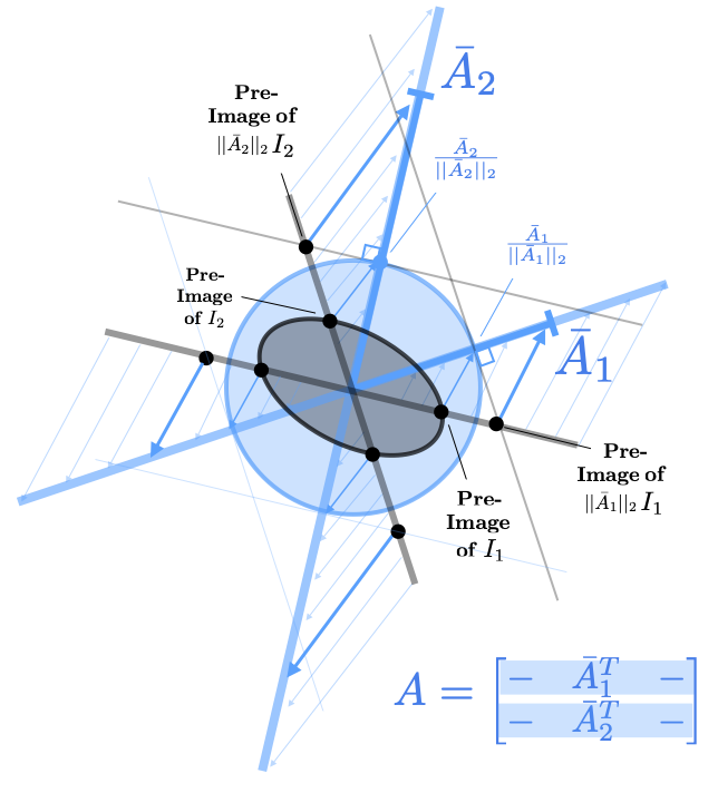
Up to a point, we can use this to visualize the action of a matrix by thinking loosely of each element of the product \( A x \) as the projection of \( x \) onto that row. This projection is best applied when \( x \) is confined to the unit ball, ie. when we think about \( x \) as a pure direction. The output element in the co-domain for a unit direction \( x \) is then given by projecting each row onto \( x \) as visualized below. Note that the longer the rows the increase in length in the output coordinate in the co-domain. We can extend this construction by then scaling each element of the resulting vector by the length of \( x \). This visualization method is not as clean as the column generation method since it suffers from sum of the difficulties of visualizating inner products in general when either of the vectors are not unit vectors.

A perhaps more insightful way to visualize row geometry is to think of directions that are orthogonal to a particular row. A column (drawn in the co-domain) clearly defines where a standard basis vector in the domain maps to (both in terms of direction and length). A row (drawn in the domain) most clearly defines an \(n-1\) dimensional subspace that is the preimage of the plane where that particular coordinate is 0 in the co-domain (or 0-plane). Note that this is purely based on the direction of the row. The length of the row gives the size of that particular output coordinate but in a slightly more subtle way (to be discussed). To see the pre-image of a particular axis in the co-domain we have to visualize the intersection of the 0-planes associated with all the other rows. This shows us the pre-image of the axis direction. (Length of vectors in this preimage are a little more subtle.) A unit vector in this direction (in the domain) is mapped to a vector (on the axis in the co-domain) with a length given by the projection of of the row onto that unit vector. All of this is visualized in the image below.
