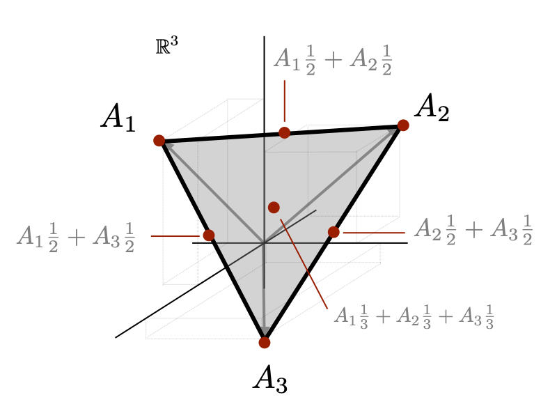
One specific type of linear combination that often arises is a convex combination. A convex combination of vectors is formed when we require the coefficients of a linear combination to all be positive and sum to one, ie. $$A_1 x_1 + A_2 x_2 + \cdots + A_n x_n, \qquad with \qquad \sum_i x_i = 1, \qquad x_i \geq 0$$ Note that we also write this constraint in more compact notation as $\mathbf{1}^Tx = 1, \ x \geq 0$ or even more simply as $x \in \Delta_n$ where $\Delta_n$ is the $n$D simplex. Visually, a convex combination of vectors live in the space between the vectors or the convex hull. For any two vectors $A_1$ and $A_2$, $A_1 \tfrac{1}{2} + A_2 \tfrac{1}{2}$ is the vector halfway between the two vectors; for $n$ vectors $\sum_i A_i \tfrac{1}{n}$ is the center of the set of vectors ("average" vector of the set); etc. Different convex combinations of vectors $\big\{A_1,A_2,A_3\big\} \in \mathbb{R}^3$ are illustrated in the figures below.

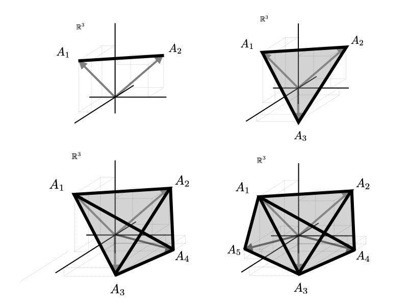
We can also show convex combinations of two, three, four, and five vectors.

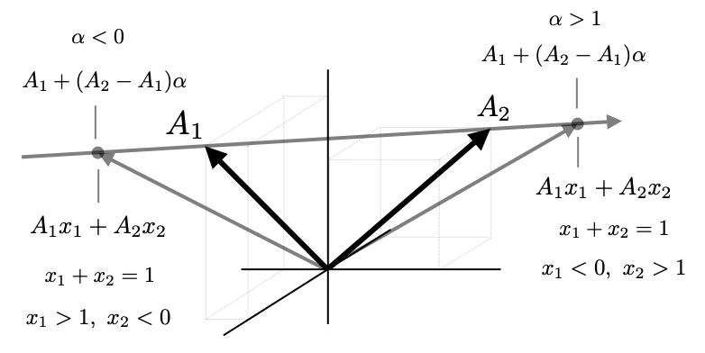
A convex combination between just two vectors is often written in the form $$y = A_1 (1-\alpha) + A_2\alpha$$ with $0 \leq \alpha \leq 1$. We notice that if we start out with $\alpha = 0$, $y=A_1$. We note that we can rearrange the above expression to show explicitly how $y$ changes with $\alpha$ $$y = A_1 + (A_2-A_1)\alpha$$ As \alpha moves from 0 to 1, $y$ starts at $A_1$ and then adds back little bits of the difference from $A_1$ to $A_2$ until $y$ reaches $A_2$. This perspective is illustrated in the figure below.

Keeping $\alpha$ between 0 and 1 keeps $y$ on the segment between $A_1$ and $A_2$. If we relax this condition and allow $\alpha$ to be negative or greater than 1, we trace out a whole line that runs through $A_1$ and $A_2$. $\alpha<0$ extends past $A_1$; $\alpha > 1$ extends off past $A_2$. Note that here $x_1 = (1-\alpha)$ and $x_2 = \alpha$. Removing the restriction on $\alpha$ is equivalent to removing the restriction that $x_1 \geq 0$ and $x_2 \geq 0$. By construction, we still have $x_1 + x_2 = (1-\alpha) + \alpha = 1$

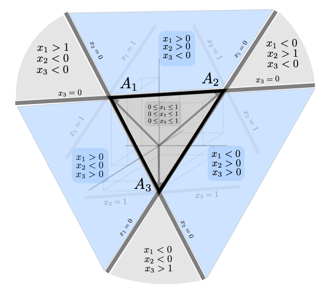
Note that this extension to the line through $A_1$ and $A_2$ applies to larger numbers of vectors as well. For example for three vectors $\big\{A_1,A_2,A_3 \big\}$, removing the restriction that $x\geq 0$ expands the convex set to the plane shown below. Note the signs of $x_1$,$x_2$, and $x_3$ in each part of the plane.