The transpose of a matrix \( A \), denoted \( A^T \), also called the adjoint of \( A \) is the matrix you get when you switch the roles of the rows and columns of \(A\). Algebraically this is quite a simple operation; we can think of the matrix values as "flipping" across the diagonal (leaving the diagonal fixed). $$ A^T = m \left\{ \begin{matrix} \\ \\ \end{matrix} \right. \underbrace{ \begin{bmatrix} A_{11} & \cdots & A_{1n} \\ \vdots & & \vdots \\ A_{m1} & \cdots & A_{mn} \end{bmatrix}_{ n }^T = \underbrace{ \begin{bmatrix} A_{11} & \cdots & A_{m1} \\ \vdots & & \vdots \\ A_{1n} & \cdots & A_{mn} \end{bmatrix} }_{m} $$ One should note that if the matrix \( A \) is not square then the dimensions of the rows and columns switch. Thus while a square matrix stays square, a tall matrix becomes fat, and a fat matrix becomes tall. The transpose operator is used in practically every linear algebraic formula. Several must know properties of transposes are listed at the end of this page.
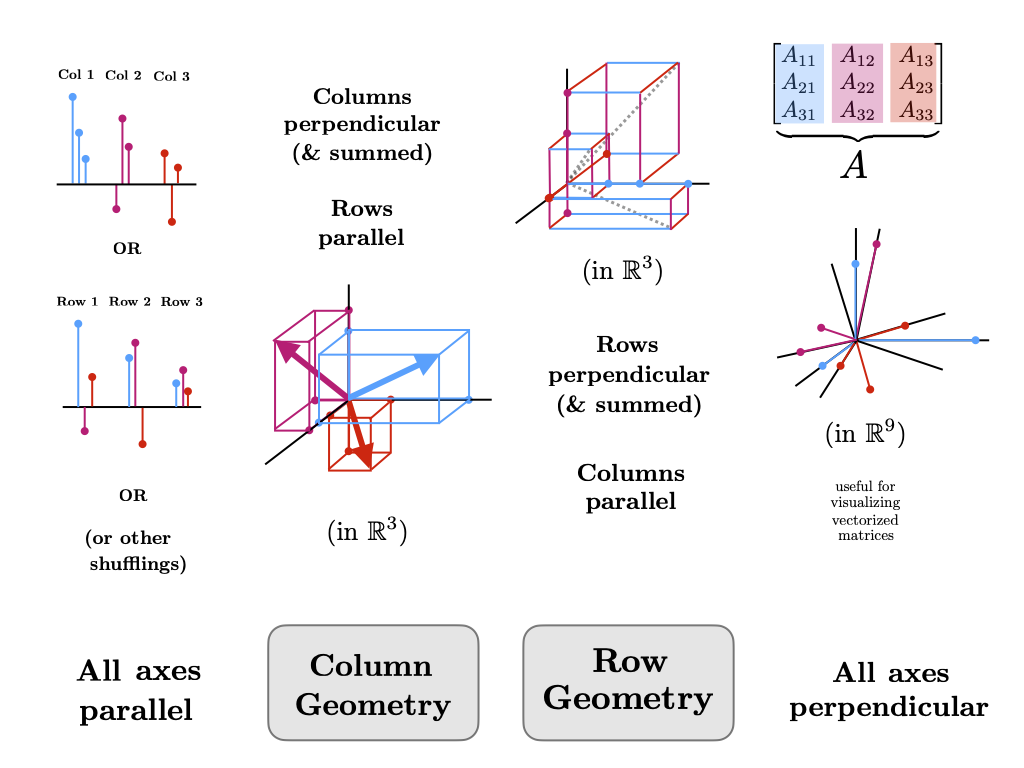
Geometrically, the transpose operation is actually profoundly deep. It is the operation that switches between the column and row geometry of a matrix. If we represent the columns of a matrix spatially (with respect to some axes for the co-domain) we also naturally give a parallel representation of the rows (along each axis in the co-domain). The transpose operation then switches the original columns to a parallel representation (along axes in the domain) and then expands the parallel representation of the rows to a spatial representation. If we visualize this operation as continuous we can get the following transformation.
It is unclear if this transformation is useful at all, but it is done in the following way.
