.dcmath - UNDER CONSTRUCTION

$$ \left[ \ \frac{\partial f}{\partial x } \ \right] = \left[ \ \frac{\partial f}{\partial g} \ \right] \left[ \ \frac{\partial g}{\partial h} \ \right] \left[ \ \frac{\partial h}{\partial x} \ \right] $$ $$ f(x) = c^Tx \quad \Rightarrow \quad \frac{\partial f}{\partial x} = c^T $$ $$ f(x) = Ax \quad \Rightarrow \quad \frac{\partial f}{\partial x} = A $$ $$ f(x) = x^TQx \quad \Rightarrow \quad \frac{\partial f}{\partial x} = x^T(Q+Q^T) = 2x^T(Q) $$ $$ f(Q) = x^TQx \quad \Rightarrow \quad \frac{\partial f}{\partial Q} = xx^T $$ $$ f(A) = y^TAx \quad \Rightarrow \quad \frac{\partial f}{\partial A} = yx^T $$

A derivative of a function \(f:x\mapsto y\) gives a linear approximation of how a perturbation in \(\Delta x\) translates into a pertubation in \(\Delta y\). The derivative notation was in fact designed by Leibniz to ellicit this idea of ratios of perturbations $$ \Delta y = \left[ \ \frac{\partial f}{\partial x} \ \right] \Delta x $$ Remembering this form can be quite useful in taking derivatives.

In order for the dimensions to work out correct, the derivative of a scalar function \(f \in \mathbb{R}\) with respect to a vector \(x \in \mathbb{R}^n\)should be an a row vector \(\frac{\partial f}{\partial x} \in \mathbb{R}^{1 \times n} \). For example for a linear function \(f:\mathbb{R}^n \rightarrow \mathbb{R}\), \(f(x) = c^Tx\) $$ \Delta y = c^T\Delta x \quad \Rightarrow \quad \frac{\partial f}{\partial x} = c^T $$

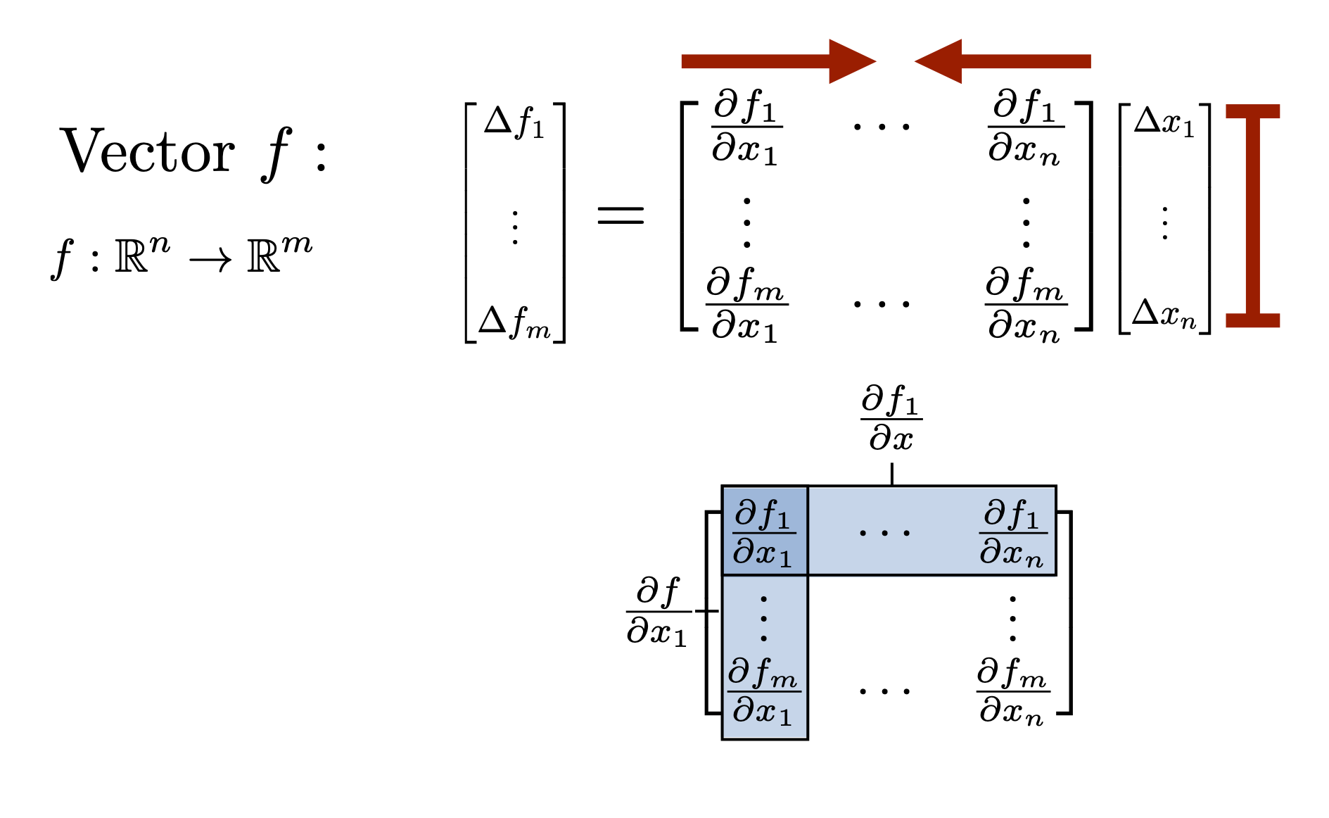
The derivative of a vector-valued function \(f \in \mathbb{R}^m\) with respect to a vector \(x \in \mathbb{R}^n\) should be an \(m \times n\) matrix \(\frac{\partial f}{\partial x} \in \mathbb{R}^{m \times n} \). For example, for linear function \(f:\mathbb{R}^n \rightarrow \mathbb{R}^m\), \(f(x) = Ax\) $$ \Delta y = A\Delta x \quad \Rightarrow \quad \left[ \ \frac{\partial f}{\partial x} \ \right] = A $$

The other critical piece is the rule of partial derivatives: to compute the full perturbation, pertub one variable at a time while holding the others fixed and then sum over all perturbations. This applies to copies of the same variable as well as totally different variables. Consider for example the quadratic function \(f:\mathbb{R}^n \rightarrow \mathbb{R}\), \(f(x) = x^TQx\). $$ \Delta y =\Delta x^T Q x + x^TQ\Delta x = (\Delta x^T Q x)^T + x^TQ\Delta x = x^T (Q^T + Q) \Delta x $$ Note that transposing scalar values can often be useful in calculations. Since \(\tfrac{1}{2}(Q+Q^T)\) is the symmetric component of \(Q\), we always assume \(Q\) is symmetric and thus we often write $$ \frac{\partial f}{\partial x} = x^T(Q+Q^T) = 2x^T(Q) $$ In the scalar case \(f:\mathbb{R}\rightarrow \mathbb{R}\) consider \(f(x) = x^2\).

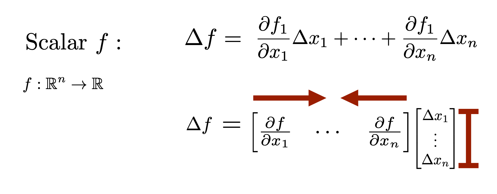
For \(f:\mathbb{R}^n \rightarrow \mathbb{R}\) $$ \Delta y = \frac{\partial f}{\partial x} \Delta x = \begin{bmatrix} \frac{\partial f}{\partial x_1} & \cdots & \frac{\partial f}{\partial x_n} \end{bmatrix} \begin{bmatrix} \Delta x_1 \\ \vdots \\ \Delta x_n \end{bmatrix} = \frac{\partial f}{\partial x_1}\Delta x_1 + \cdots + \frac{\partial f}{\partial x_n}\Delta x_n $$

For \(f:\mathbb{R}^n \rightarrow \mathbb{R}^m\) $$ f(x) = \begin{bmatrix} f_1(x) \\ \vdots \\ f_m(x) \end{bmatrix} \quad \Rightarrow \quad \left[ \ \frac{\partial f}{\partial x} \ \right] = \begin{bmatrix} - & \frac{\partial f_1}{\partial x} & - \\ & \vdots & \\ - & \frac{\partial f_m}{\partial x} & - \end{bmatrix} = \begin{bmatrix} \frac{\partial f_1}{\partial x_1} & \cdots & \frac{\partial f_1}{\partial x_n} \\ \vdots & & \vdots \\ \frac{\partial f_m}{\partial x_1} & \cdots & \frac{\partial f_m}{\partial x_n} \end{bmatrix} $$

The above shows that derivatives should always be conceptualized as row vectors (covectors). If this is done, the chain rule can often be applied in a straightforward manner. Consider the composition of functions \( f(g(h(x))) \). The chain rule gives that $$ \Delta y = \left[ \ \frac{\partial f}{\partial x} \ \right] \Delta x = \left[ \ \frac{\partial f}{\partial g} \ \right] \left[ \ \frac{\partial g}{\partial h} \ \right] \left[ \ \frac{\partial h}{\partial x} \ \right] \Delta x $$ Note that the dimensions work out correctly. For example if \(f:\mathbb{R}^k \rightarrow \mathbb{R}^m \), \(g:\mathbb{R}^l \rightarrow \mathbb{R}^k \), and \(h:\mathbb{R}^n \rightarrow \mathbb{R}^l \), then $$ \frac{\partial f}{\partial g} \in \mathbb{R}^{m \times k}, \quad \frac{\partial g}{\partial h} \in \mathbb{R}^{k \times l}, \quad \frac{\partial h}{\partial x} \in \mathbb{R}^{l \times n} \quad \Rightarrow \quad \left[ \ \frac{\partial f}{\partial x } \ \right] = \left[ \ \frac{\partial f}{\partial g} \ \right] \left[ \ \frac{\partial g}{\partial h} \ \right] \left[ \ \frac{\partial h}{\partial x} \ \right] \in \mathbb{R}^{m \times n} $$

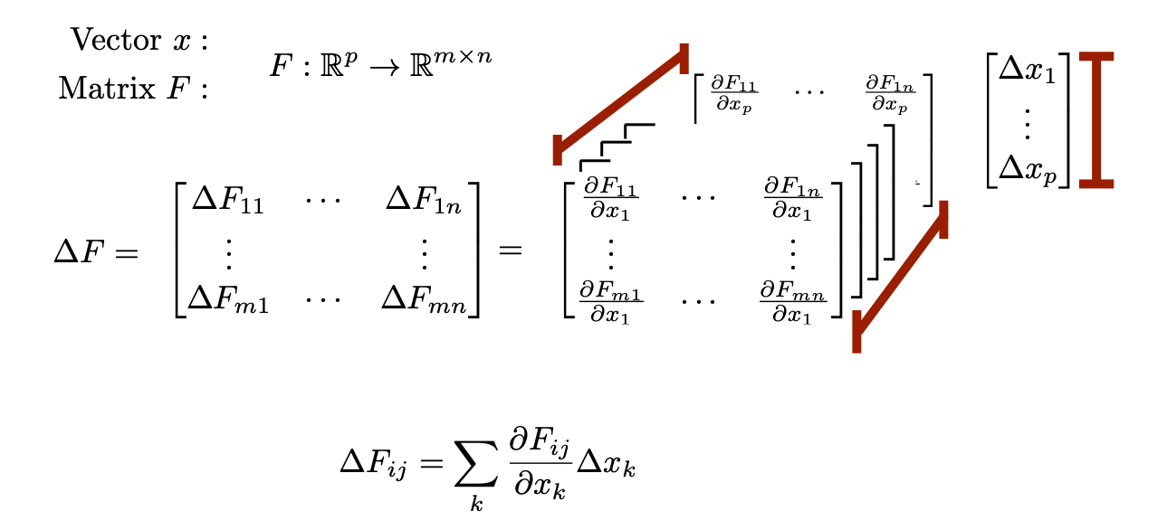
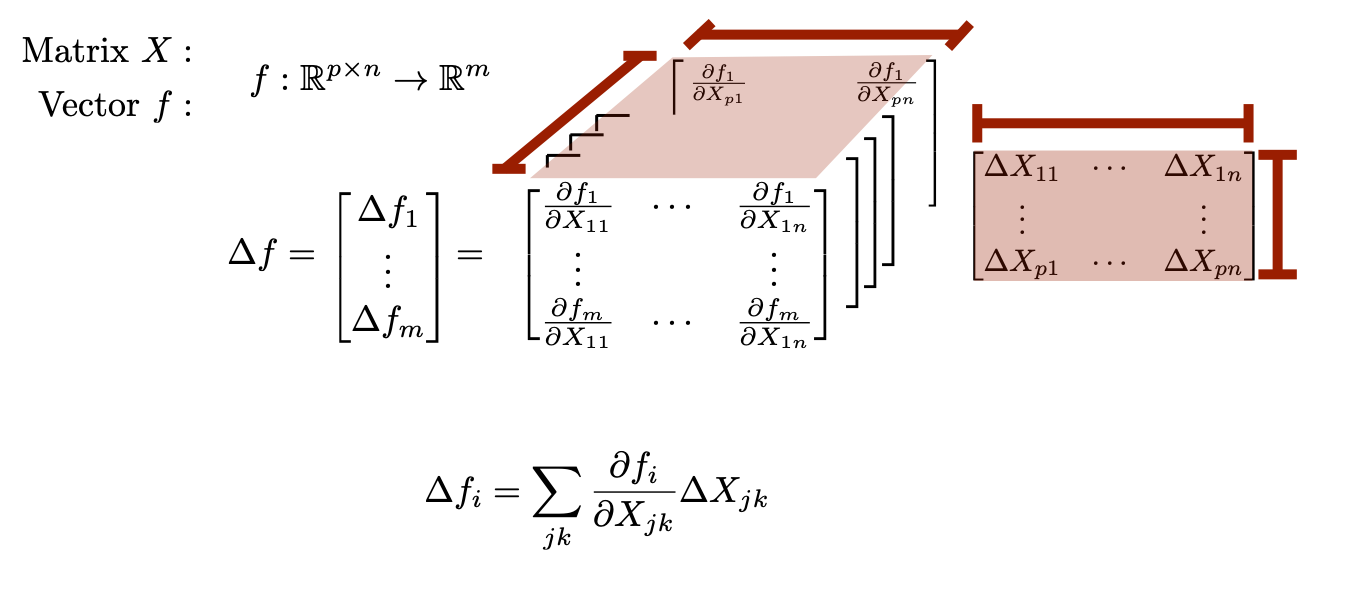
Writing the deritives for functions of matrices such as \(f:\mathbb{R}^{m \times n} \rightarrow \mathbb{R}^m\) (ex: \(f(X) = Xz\)) or \(f:\mathbb{R}^{m \times n} \rightarrow \mathbb{R}^{k \times n}\) (ex. \(f(X) = AX\)) are difficult to write because technically they are best represented as 3-tensors and 4-tensors respectively. This leaves two options.

1) Store the derivative as the appropriate tensor. Perturbation computations must then be written using sums or Einstein summation notation. For example \(Y=F(X)\) $$ \Delta Y_{kl} = \sum_{ij}\frac{\partial F_{kl}}{\partial X_{ij}} \Delta X_{ij} = \frac{\partial F}{\partial X}_{klij} \Delta X_{ij} $$ 2) Flatten out the tensor by vectorizing each matrix and writing the derivative as a large matrix (see below).

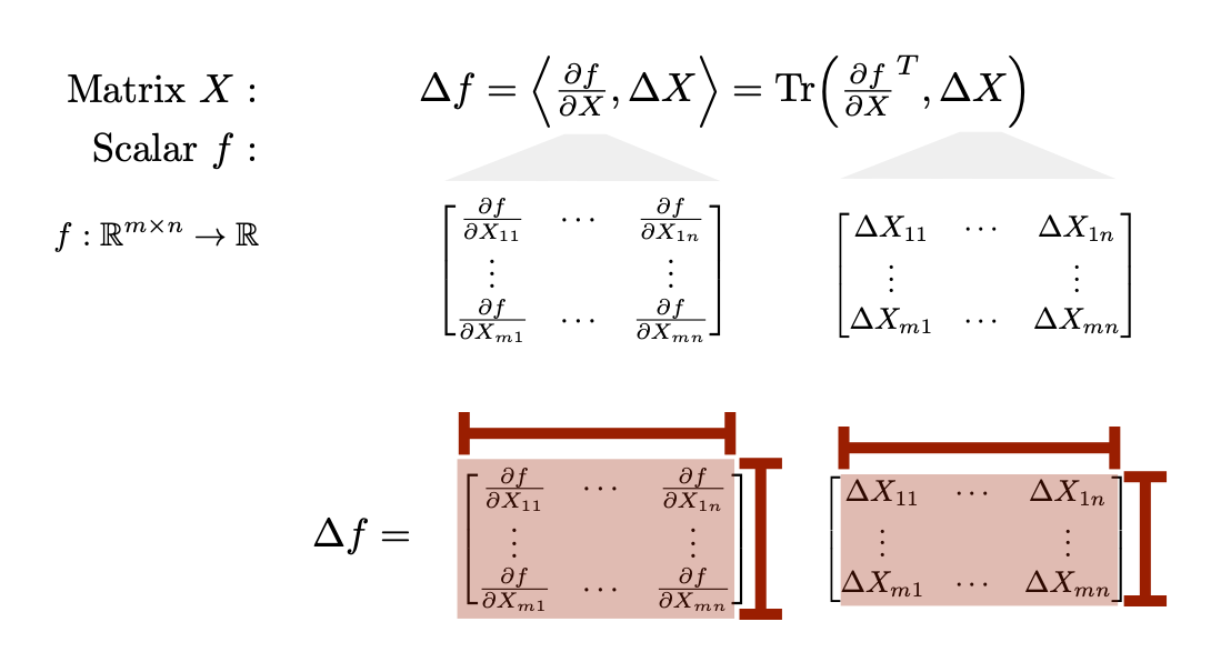
The one exception is for scalar-valued functions of matrices. In tensor form for \(y = f(X)\) \(f:\mathbb{R}^{m \times n} \rightarrow \mathbb{R} \), \(\frac{\partial f}{\partial X} is simply a 2-tensor and so we can still store it easily as a matrix. (Alternatively, if the input matrix is vectorized, the derivative will be a row vector.) Using the trace to represent matrix inner products is conceptually and computationally useful in these cases. Analogous to the function \(f(x)=c^Tx=\sum_i c_ix_i\) for matrices we often have functions of the form \(f(X) = \sum_{ij}C_{ij}X_{ij}\) which can be represented compactly using the trace operator $$ f(X) = \sum_{ij}C_{ij}X_{ij} = Tr(C^TX) $$ Along these lines, the inner-product between two matrices is often given by \(\langle C,X\rangle = Tr(C^TX)\). As a result a perturbation analysis would given $$ \Delta f = \langle \frac{\partial f}{\partial X}, \Delta X \rangle = Tr(C^T \Delta X) $$ and thus \(\frac{\partial f}{\partial X} = C\). Elementwise, we have that \(\frac{\partial f}{\partial X_{ij}} = C_{ij}\). This trace form can be quite useful for algebraic manipulations (since traces are quite pleasantly behaved algebraically) as illustrated by the following examples. examples illustrate $$ f(Q) = x^TQx = Tr(x^TQx) = Tr(xx^TQ) \quad \Rightarrow \quad \frac{\partial f}{\partial Q} = xx^T $$ $$ f(A) = y^TAx = Tr(y^TAx) = Tr(xy^TA) \quad \Rightarrow \quad \frac{\partial f}{\partial A} = yx^T $$

(NEEDS TO BE ADDED)