(An interactive version of this gif is given at the end of this post.)

Shortest Path LP

In two previous posts, we gave visualizations of the simplex method and also several results on incidence matrices of graphs. Using a node-edge incidence matrix, we can formulate a weighted shortest path problem as a linear program and solve it using the simplex method. In this post, we detail this optimization problem and give visualizations. We note at the outset that this not necessarily a computationally efficient way to solve a shortest path problem (Dijkstra's algorithm is much better), but it does provide interesting insights into the geometry of graph flow constraints as well as the simplex method.

Optimization Formulation

We consider a graph \(\mathcal{G}=(\mathcal{V},\mathcal{E})\) with nodes \(\mathcal{V}\) and edges \(\mathcal{E}\) and an origin node \(o\) and a destination node \(d\). We can frame the weighted shortest path optimization problem from \(o\) to \(d\) as $$ \begin{aligned} \min_x & \quad c^\top x \\ \text{s.t.} & \quad Ex = S, \ x \geq 0 \end{aligned} $$ Here, \(x \in \mathbb{R}^{|\mathcal{E}|}\) is an edge-flow vector that at optimum will become an indicator vector for the shortest path. ) and \(c \in \mathbb{R}_+^{|\mathcal{E}|}\) is a vector of costs or weights on each of the edges. The objective \(c^\top x\) gives the overall cost incurred by an edge flow vector \(x\). \(E \in \mathbb{R}^{|\mathcal{V}|\times |\mathcal{E}|}\) is the node-edge incidence matrix of the graph detailed in our previous post post. \(S \in \mathbb{R}^{|\mathcal{V}|}\) is a source-sink vector with a -1 at the origin and a 1 at the destination. $$ \begin{aligned} E_{ij} = \begin{cases} -1 & \text{ if edge \(j\) starts at node \(i\) } \\ 1 & \text{ if edge \(j\) ends at node \(i\) } \\ 0 & \text{ otherwise} \end{cases}, \qquad S_i = \begin{cases} -1 & \text{ at the origin node } \\ 1 & \text{ at the destination node } \\ 0 & \text{ otherwise} \end{cases}, \end{aligned} $$

Intuitively for a fully connected graph, this optimization problem routes one unit of mass from the origin node to the destination node (with mass conserved at all the other nodes) in such as to minimize the cost incurred. Technically each element of \(x\) can be a fraction less than 1. This comes from the fact that we are working with a continuous relaxation of shortest path problem. Fractional values of \(x\) can be interpreted fraction of times or probability of traversing a particular edge if a stochastic path planning problem is used using only optimal edges. At the optimum, however, since it is a linear program any route with positive mass on each edge will be optimal and generically only a single route will have mass. One should also note that this constraint allows \(x\) to contain components in the cycle space of the graph. However, the optimal solution will not contain any component in the cycle space since for positive \(x\) and positive \(c\) any cycle component would simply increase the cost unnecessarily, ie. no one makes a loop while traversing a shortest path.

Caveat: Reducing the incidence matrix

There is one problem with the above program: the incidence matrix by nature has redundant constraints. This comes from the fact that each column sums to 1. Intuitively, if we enforce mass conservation at all but one node then that ensures mass conservation at the final node as well. In the above problem, we can take care of this by simply removing the row corresponding to any node from the constraint \(Ex=S\). We will do this in the following and make several comments about it's effect on the problem as we go along.

The Simplex Method Tableau

We note that our shortest path problem is already in canonical form for applying the simplex method - all our variables are positive and we do not need any extra slack variables. We an write out our canonical tableau as follows $$ \begin{aligned} \begin{bmatrix} 1 & c^\top & 0 \\ 0 & E & S \end{bmatrix} \end{aligned} $$ Here we will not take \(E\) and \(S\) to be the incidence matrix and source-sink vector exactly but rather the incidence matrix and source-sink vector wiht one row removed so that the constraint \(Ex=S\) is full row rank. We will choose to remove the destination node. The constraint now reads that one unit of flow mass enters the graph at the origin node and is conserved everywhere else except the destination. The constraint therefore will cause all the mass to flow to the destination node (and out of the graph).

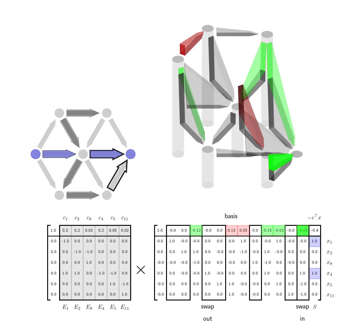
Any basis we choose will have \(|\mathcal{V}|-1\) columns. Assuming (WLOG) that the first set of columns are linearly independent, we can segment \(E\) and \(c\) as into the first \(|\mathcal{V}|-1\) columns and the remaining columns, \(E = \big[ E_1 \ E_2 \big]\) and \(c^\top = [ c_1^\top \ c_2^\top ]\) We can write our initial basis matrix which we will denote as \(B \in \mathbb{R}^{|\mathcal{V}|\times |\mathcal{V}|}\) and it's inverse as $$ \begin{aligned} B = \begin{bmatrix} 1 & c_1^\top \\ 0 & E_1 \end{bmatrix} \qquad B^{-1} = \begin{bmatrix} 1 & v^\top \\ 0 & E_1^{-1} \end{bmatrix} , \quad \text{with \quad} v^\top = -c_1^\top E_1^{-1} \end{aligned} $$ This form of the inverse can be easily derived from the block matrix inversion lemma or one can just quickly check that it is correct. We can then write our tableau as $$ \begin{aligned} \begin{bmatrix} 1 & c^\top & 0 \\ 0 & E & S \end{bmatrix} & = \begin{bmatrix} 1 & c_1^\top & c_2^\top& 0 \\ 0 & E_1 & E_2 & S \end{bmatrix} \\ & = \begin{bmatrix} 1 & c_1^\top \\ 0 & E_1 \end{bmatrix} \begin{bmatrix} 1 & 0 & c_2^\top + v^\top E_2 & 0 \\ 0 & I & E_1^{-1}E_2 & S \end{bmatrix} \\ \end{aligned} $$

Interpretation via Tree-Cycle Decomposition

We can make several important comments. First, the condition that \(E_1\) is invertible is equivalent to making sure that \(E_1\) is the incidence matrix for a spanning tree of the graph. It has \(|\mathcal{V}|-1\) edges as expected. By removing the destination node, we have made sure that \(E_1\) is square. \(E_1\) will be invertible if and only if it has only a trivial nullspace which is equivalent to the subgraph corresponding to \(E_1\) having no cycles, ie. a spanning tree. Next we note that in row reducing the tableau above, we have implicitly used the tree-cycle decomposition of the incidence matrix. $$ \begin{aligned} E = E_1 \Big[ I \ \ E_1^{-1}E_2 \Big] \end{aligned} $$ Here as just stated \(E_1\) is a spanning tree and each of the other edges in \(E_2\) correspond to a cycle in the graph as discussed in the previous post. Each time we select a new basis for the tableau we are selecting a different spanning tree for the graph. At any given step, the spanning tree we have is our current guess for what is the lowest cost way to travel between any of the nodes in the graph, ie. using the edges in the spanning tree. When we've finished the algorithm, we will have the lowest weight spanning tree. For any edge not in the spanning tree, there are two ways to get between the start and end node of that edge. The first is simply to take the edge; the second is to the go the other way around the cycle, using only edges in the spanning tree. The term \(E_1^{-1}E_2 \) is the coordinates of this alternative walk around the cycle relative to the edges in the spanning tree. The vector \(c_2\) contains the cost of traveling any of the non-spanning tree edges; the term \(c_1^\top E_1^{-1}E_2\) contains the cost of making the same transition from the start to end node via edges in the spanning tree. At each step of the algorithm, we want to add an edge to the spanning tree that reduces the cost of travel in the spanning tree. We can do this by comparing these two costs in \(c_2\) and \(c_1^\top E_1^{-1}E_2\) and picking an element where the new edge is faster. Indeed, this is exactly the term that we see show up in the tableau $$ \begin{aligned} c_2^\top - c_1^\top E_1^{-1}E_2 \end{aligned} $$ Since we are minimizing we want to swap in basis columns where the top row is negative, ie, where the element of \(c_2\) is less than the element in \(c_1^\top E_1 ^{-1}E_2\). When we choose which column to swap out, the rules from the simplex method will simply ensure that the basis edges form a spanning tree, ie. the columns of the new \(E_1\) are linearly independent, and also that there is still a path vector \(x\) from the origin to the destination that is positive in each element, ie. respects the orientation of the graph edges.

Visualization: Cost-to-go as Height of Nodes

Intuitively the above explanation gives a clear picture of what the simplex method is doing in this case, swapping in and out edges to find the minimum cost spanning tree. There is one more variable that is interesting from an optimization and visualization perspective, \(v^\top = - c_1^\top E_1^{-1}\). This vector \(v\) can be thought of as the cost-to-go with the current spanning tree. To be explicit the term \(v^\top E_2 \) takes the difference of the values of \(v\) between any two start and end nodes. That difference is equivalent to the cost of traversing between those two nodes within the spanning tree. If we represent the values in \(v\) as the height of the nodes we then we can visually see whether or a potential new edge that we might want to add is efficient or not. If the cost associated with the edge is greater than the current height difference between the nodes than the edge is inefficient and should not be added. If, however, the edge cost is less than the current height difference the edge is a good candidate for being added to the spanning tree. We show this visualization idea here. The heights of the nodes here correspond to \(v^\top \) as discussed. The lengths of hte black vertical rectangles correspond to the cost of the edge. If taking a particular edge costs less than the current cost to go estimate then the edge is highlighted in green. If not, it is highlighted in red.

We animate the full simplex method process here.

We now apply the same technique to a larger graph (without showing the incidence matrix) and highlight each edge as we swap them in and out. Note that the simplex method is trying to find the lowest cost spanning tree for the whole graph, so it often swaps in and out edges that don't have an immediate impact on current shortest path.